Unsteady Flow Operations

Overview

This notebook demonstrates reading and manipulating unsteady flow files (.u## format). These define time-varying boundary conditions and simulation parameters.

What You'll Learn

• Parse unsteady flow file structure
• Extract boundary condition time series
• Modify initial condition lines
• Update simulation parameters

LLM Forward Approach

• Verification: Compare to HEC-RAS GUI
• Audit Trail: Save modified flow files
• Reproducibility: Document parameter changes

Reference Documentation

• HEC-RAS User's Manual, Chapter 7: Entering Flow Data
• HEC-RAS Hydraulic Reference Manual

Python

# =============================================================================
# DEVELOPMENT MODE TOGGLE
# =============================================================================
USE_LOCAL_SOURCE = True  # <-- TOGGLE THIS

if USE_LOCAL_SOURCE:
    import sys
    from pathlib import Path
    local_path = str(Path.cwd().parent)
    if local_path not in sys.path:
        sys.path.insert(0, local_path)
    print(f"📁 LOCAL SOURCE MODE: Loading from {local_path}/ras_commander")
else:
    print("📦 PIP PACKAGE MODE: Loading installed ras-commander")

# Import ras-commander
from ras_commander import HdfResultsXsec, RasCmdr, RasExamples, RasPlan, RasPrj, RasUnsteady, init_ras_project, ras

# Additional imports
import os
import numpy as np
import pandas as pd
from IPython.display import display
import matplotlib.pyplot as plt

# Verify which version loaded
import ras_commander
print(f"✓ Loaded: {ras_commander.__file__}")

# Set to True to generate plots, False to skip plotting
generate_plots = True
# Plot label helpers for technical figures
PLOT_LABELS = {
    "Water_Surface": {"title": "Water Surface Elevation", "ylabel": "Water Surface Elevation (ft NAVD88)"},
    "Velocity_Total": {"title": "Total Velocity", "ylabel": "Velocity (ft/s)"},
    "Velocity_Channel": {"title": "Channel Velocity", "ylabel": "Velocity (ft/s)"},
    "Flow_Lateral": {"title": "Lateral Flow", "ylabel": "Flow (cfs)"},
    "Flow": {"title": "Cross-Section Flow", "ylabel": "Flow (cfs)"},
}


def annotate_peak(ax, x_values, y_values, label="Peak", offset=(18, -28), color="#b3261e"):
    values = np.asarray(y_values, dtype=float)
    if values.size == 0 or np.all(np.isnan(values)):
        return
    y_min = float(np.nanmin(values))
    y_max = float(np.nanmax(values))
    y_span = y_max - y_min
    if y_span == 0 and abs(y_max) < 1e-9:
        ax.text(
            0.02,
            0.90,
            "No lateral flow (0 cfs)",
            transform=ax.transAxes,
            fontsize=9,
            color="#444444",
            bbox={"boxstyle": "round,pad=0.25", "fc": "white", "ec": "#bbbbbb", "alpha": 0.9},
        )
        ax.set_ylim(-0.05, 0.05)
        return
    peak_idx = int(np.nanargmax(values))
    peak_y = float(values[peak_idx])
    peak_x = x_values[peak_idx]
    ax.scatter([peak_x], [peak_y], color=color, s=36, zorder=3)
    ax.annotate(
        f"{label}: {peak_y:,.1f}",
        xy=(peak_x, peak_y),
        xytext=offset,
        textcoords="offset points",
        arrowprops={"arrowstyle": "->", "color": "#444444", "lw": 1.0},
        fontsize=9,
        ha="left",
        va="top",
        annotation_clip=True,
    )

Text Only

📁 LOCAL SOURCE MODE: Loading from C:\GH\symphony-workspaces\ras-commander\CLB-888/ras_commander


2026-06-03 15:12:37 - numexpr.utils - INFO - NumExpr defaulting to 8 threads.


✓ Loaded: C:\GH\symphony-workspaces\ras-commander\CLB-888\ras_commander\__init__.py

Parameters

Configure these values to customize the notebook for your project.

Python

# =============================================================================
# PARAMETERS - Edit these to customize the notebook
# =============================================================================
from pathlib import Path

# Project Configuration
PROJECT_NAME = "Muncie"           # Example project to extract
RAS_VERSION = "7.0"               # HEC-RAS version (6.3, 6.5, 6.6, etc.)

# Execution Settings
PLAN = "01"                       # Plan number to execute
NUM_CORES = 4                     # CPU cores for 2D computation
RUN_SUFFIX = "run"                # Suffix for run folder (e.g., Muncie_run)

Python

import os
import sys
import logging
from contextlib import contextmanager
from pathlib import Path
import numpy as np
import pandas as pd
from IPython.display import display
import matplotlib.pyplot as plt


@contextmanager
def temporary_logger_level(logger_name, level):
    """Temporarily raise a logger threshold for notebook cells that intentionally initialize noisy example projects."""
    target_logger = logging.getLogger(logger_name)
    previous_level = target_logger.level
    target_logger.setLevel(level)
    try:
        yield
    finally:
        target_logger.setLevel(previous_level)

# Set to True to generate plots, False to skip plotting
generate_plots = True

Understanding Unsteady Flow Files in HEC-RAS

Unsteady flow files (.u* files) in HEC-RAS define the time-varying boundary conditions that drive dynamic simulations. These include:

• Flow Hydrographs: Time-series of flow values at model boundaries
• Stage Hydrographs: Time-series of water surface elevations
• Lateral Inflows: Distributed inflows along a reach
• Gate Operations: Time-series of gate settings
• Meteorological Data: Rainfall, evaporation, and other meteorological inputs

The RasUnsteady class in RAS Commander provides methods for working with these files, including extracting boundaries, reading tables, and modifying parameters.

Let's set up our working directory and define paths to example projects:

Downloading and Extracting Example HEC-RAS Projects

We'll use the RasExamples class to download and extract an example HEC-RAS project with unsteady flow files. For this notebook, we'll use the project specified in the parameters (default: Muncie).

Python

# Extract the example project
# The extract_project method downloads the project from GitHub if not already present,
# and extracts it to the example_projects folder
project_path = RasExamples.extract_project(PROJECT_NAME, suffix="300")
print(f"Extracted project to: {project_path}")  


# Verify the path exists
print(f"Project exists: {project_path.exists()}")

Text Only

2026-06-03 15:12:39 - ras_commander.RasExamples - INFO - Successfully extracted project 'Muncie' to C:\GH\symphony-workspaces\ras-commander\CLB-888\examples\example_projects\Muncie_300


Extracted project to: C:\GH\symphony-workspaces\ras-commander\CLB-888\examples\example_projects\Muncie_300
Project exists: True

Step 1: Project Initialization

The first step is to initialize the HEC-RAS project. This is done using the init_ras_project() function, which takes the following parameters:

• ras_project_folder: Path to the HEC-RAS project folder (required)
• ras_version: HEC-RAS version (e.g., "6.6") or path to Ras.exe (required first time)

This function initializes the global ras object that we'll use for the rest of the notebook.

Python

# Initialize the HEC-RAS project
# This function returns a RAS object, but also updates the global 'ras' object
# Parameters:
#   - ras_project_folder: Path to the HEC-RAS project folder
#   - ras_version: HEC-RAS version or path to Ras.exe

init_ras_project(project_path, RAS_VERSION)
print(f"Initialized HEC-RAS project: {ras.project_name}")

# Display the unsteady flow files in the project

Text Only

2026-06-03 15:12:39 - ras_commander.RasUtils - INFO - Discovered HEC-RAS 7.0 at C:\Program Files (x86)\HEC\HEC-RAS\7.0\Ras.exe via filesystem (x86)


2026-06-03 15:12:39 - ras_commander.RasUtils - INFO - Discovered HEC-RAS 6.7 Beta 5 at C:\Program Files (x86)\HEC\HEC-RAS\6.7 Beta 5\Ras.exe via filesystem (x86)


2026-06-03 15:12:39 - ras_commander.RasUtils - INFO - Discovered HEC-RAS 6.7 Beta 4 at C:\Program Files (x86)\HEC\HEC-RAS\6.7 Beta 4\Ras.exe via filesystem (x86)


2026-06-03 15:12:39 - ras_commander.RasUtils - INFO - Discovered HEC-RAS 6.6 at C:\Program Files (x86)\HEC\HEC-RAS\6.6\Ras.exe via filesystem (x86)


2026-06-03 15:12:39 - ras_commander.RasUtils - INFO - Discovered HEC-RAS 6.5 at C:\Program Files (x86)\HEC\HEC-RAS\6.5\Ras.exe via filesystem (x86)


2026-06-03 15:12:39 - ras_commander.RasUtils - INFO - Discovered HEC-RAS 6.4.1 at C:\Program Files (x86)\HEC\HEC-RAS\6.4.1\Ras.exe via filesystem (x86)


2026-06-03 15:12:39 - ras_commander.RasUtils - INFO - Discovered HEC-RAS 6.3.1 at C:\Program Files (x86)\HEC\HEC-RAS\6.3.1\Ras.exe via filesystem (x86)


2026-06-03 15:12:39 - ras_commander.RasUtils - INFO - Discovered HEC-RAS 6.3 at C:\Program Files (x86)\HEC\HEC-RAS\6.3\Ras.exe via filesystem (x86)


2026-06-03 15:12:39 - ras_commander.RasUtils - INFO - Discovered HEC-RAS 6.2 at C:\Program Files (x86)\HEC\HEC-RAS\6.2\Ras.exe via filesystem (x86)


2026-06-03 15:12:39 - ras_commander.RasUtils - INFO - Discovered HEC-RAS 6.1 at C:\Program Files (x86)\HEC\HEC-RAS\6.1\Ras.exe via filesystem (x86)


2026-06-03 15:12:39 - ras_commander.RasUtils - INFO - Discovered HEC-RAS 6.0 at C:\Program Files (x86)\HEC\HEC-RAS\6.0\Ras.exe via filesystem (x86)


2026-06-03 15:12:39 - ras_commander.RasUtils - INFO - Discovered HEC-RAS 5.0.7 at C:\Program Files (x86)\HEC\HEC-RAS\5.0.7\Ras.exe via filesystem (x86)


2026-06-03 15:12:39 - ras_commander.RasUtils - INFO - Discovered HEC-RAS 5.0.6 at C:\Program Files (x86)\HEC\HEC-RAS\5.0.6\Ras.exe via filesystem (x86)


2026-06-03 15:12:39 - ras_commander.RasUtils - INFO - Discovered HEC-RAS 5.0.5 at C:\Program Files (x86)\HEC\HEC-RAS\5.0.5\Ras.exe via filesystem (x86)


2026-06-03 15:12:39 - ras_commander.RasUtils - INFO - Discovered HEC-RAS 5.0.4 at C:\Program Files (x86)\HEC\HEC-RAS\5.0.4\Ras.exe via filesystem (x86)


2026-06-03 15:12:39 - ras_commander.RasUtils - INFO - Discovered HEC-RAS 5.0.3 at C:\Program Files (x86)\HEC\HEC-RAS\5.0.3\Ras.exe via filesystem (x86)


2026-06-03 15:12:39 - ras_commander.RasUtils - INFO - Discovered HEC-RAS 5.0.1 at C:\Program Files (x86)\HEC\HEC-RAS\5.0.1\Ras.exe via filesystem (x86)


2026-06-03 15:12:39 - ras_commander.RasUtils - INFO - Discovered HEC-RAS 5.0 at C:\Program Files (x86)\HEC\HEC-RAS\5.0\Ras.exe via filesystem (x86)


2026-06-03 15:12:39 - ras_commander.RasUtils - INFO - Discovered HEC-RAS 4.1.0 at C:\Program Files (x86)\HEC\HEC-RAS\4.1.0\Ras.exe via filesystem (x86)


2026-06-03 15:12:39 - ras_commander.RasUtils - INFO - Discovered HEC-RAS 4.0 at C:\Program Files (x86)\HEC\HEC-RAS\4.0\Ras.exe via filesystem (x86)


2026-06-03 15:12:39 - ras_commander.RasUtils - INFO - Discovered 20 installed HEC-RAS version(s)


2026-06-03 15:12:39 - ras_commander.RasPrj - INFO - HEC-RAS 7.0 found via version discovery: C:\Program Files (x86)\HEC\HEC-RAS\7.0\Ras.exe


2026-06-03 15:12:39 - ras_commander.RasMap - INFO - Successfully parsed RASMapper file: C:\GH\symphony-workspaces\ras-commander\CLB-888\examples\example_projects\Muncie_300\Muncie.rasmap


2026-06-03 15:12:39 - ras_commander.RasPrj - INFO - ras-commander v0.98.0 | An open-source project of CLB Engineering Corporation (https://clbengineering.com/) | Docs: https://ras-commander.readthedocs.io | GitHub: https://github.com/gpt-cmdr/ras-commander


2026-06-03 15:12:39 - ras_commander.RasPrj - INFO - Project initialized: Muncie | Folder: C:\GH\symphony-workspaces\ras-commander\CLB-888\examples\example_projects\Muncie_300


2026-06-03 15:12:39 - ras_commander.RasPrj - INFO - Using HEC-RAS executable: C:\Program Files (x86)\HEC\HEC-RAS\7.0\Ras.exe


2026-06-03 15:12:39 - ras_commander.RasPrj - INFO - 
═══════════════════════════════════════════════════════════════════════
ras-commander | HEC-RAS Automation Library
Docs: https://gpt-cmdr.github.io/ras-commander/
Repo: https://github.com/gpt-cmdr/ras-commander
═══════════════════════════════════════════════════════════════════════

PROJECT DATAFRAMES (single source of truth — use these, not file globbing):
  ras.plan_df        Plans, HDF paths, geometry/flow associations
  ras.geom_df        Geometry files and HDF preprocessor paths
  ras.flow_df        Steady flow files
  ras.unsteady_df    Unsteady flow files and configurations
  ras.boundaries_df  Boundary conditions (type, name, location)
  ras.results_df     Lightweight HDF results summaries
  ras.rasmap_df      RASMapper layers, terrain, land cover paths

KEY APIS (static classes — call directly, never instantiate):
  Execution:    RasCmdr.compute_plan() / compute_parallel() / compute_test_mode()
  Plan Files:   RasPlan.clone_plan() / clone_geom() / set_geom()
  Unsteady:     RasUnsteady — IC/BC management, gate openings, precipitation
  Geometry:     GeomCrossSection, GeomBridge, GeomStorage, GeomLateral, GeomMesh
  HDF Results:  HdfResultsPlan.get_wse() / get_compute_messages()
                HdfResultsMesh.get_mesh_max_ws() / get_mesh_cells_timeseries()
                HdfMesh.get_mesh_cell_points()
  QA/QC:        RasCheck.run_check() / RasFixit (geometry repair)
  DSS:          RasDss.get_timeseries() / check_pathname()
  USGS:         UsgsGaugeSpatial, GaugeMatcher, RasUsgsBoundaryGeneration
  Precipitation: StormGenerator, Atlas14Storm, PrecipAorc, Atlas14Variance
  Terrain:      RasTerrain.create_terrain_hdf() / RasTerrainMod

MULTI-PROJECT: Pass ras_object= to all API calls when using local RasPrj instances.

EXAMPLES: 100+ notebooks in examples/ (100s=execution, 200s=geometry, 300s=unsteady,
  400s=HDF results, 500s=remote, 800s=QA/QC, 900s=data integration).
  Review relevant notebooks before assembling new workflows.

PLATFORM: Most HEC-RAS operations require Windows. Linux/Wine support for
  headless execution, data access, geometry modification, and preprocessing
  is available via RasProcess (HEC-RAS 6.6+). See ras_commander/RasProcess.py.
  Remote distributed execution: ras_commander/remote/ (PsExec, Docker, SSH, cloud).
═══════════════════════════════════════════════════════════════════════


Initialized HEC-RAS project: Muncie

Python

print("\nHEC-RAS Project Plan Data (plan_df):")
ras.plan_df

Text Only

HEC-RAS Project Plan Data (plan_df):

	plan_number	unsteady_number	geometry_number	Plan Title	Program Version	Short Identifier	Simulation Date	Computation Interval	Mapping Interval	Run HTab	...	Friction Slope Method	UNET D2 SolverType	UNET D2 Name	HDF_Results_Path	Geom File	Geom Path	Flow File	Flow Path	full_path	flow_type
0	01	01	01	Unsteady Multi  9-SA run	5.00	9-SAs	02JAN1900,0000,02JAN1900,2400	15SEC	5MIN	1	...	1	NaN	NaN	None	01	C:\GH\symphony-workspaces\ras-commander\CLB-88...	01	C:\GH\symphony-workspaces\ras-commander\CLB-88...	C:\GH\symphony-workspaces\ras-commander\CLB-88...	Unsteady
1	03	01	02	Unsteady Run with 2D 50ft Grid	5.10	2D 50ft Grid	02JAN1900,0000,02JAN1900,2400	10SEC	5MIN	-1	...	1	Pardiso (Direct)	2D Interior Area	None	02	C:\GH\symphony-workspaces\ras-commander\CLB-88...	01	C:\GH\symphony-workspaces\ras-commander\CLB-88...	C:\GH\symphony-workspaces\ras-commander\CLB-88...	Unsteady
2	04	01	04	Unsteady Run with 2D 50ft User n Value R	5.10	50ft User n Regions	02JAN1900,0000,02JAN1900,2400	10SEC	5MIN	1	...	1	Pardiso (Direct)	2D Interior Area	None	04	C:\GH\symphony-workspaces\ras-commander\CLB-88...	01	C:\GH\symphony-workspaces\ras-commander\CLB-88...	C:\GH\symphony-workspaces\ras-commander\CLB-88...	Unsteady

3 rows × 35 columns

Python

print("\nHEC-RAS Project Geometry Data (geom_df):")
ras.geom_df

Text Only

HEC-RAS Project Geometry Data (geom_df):

	geom_file	geom_number	full_path	hdf_path	has_1d_xs	has_2d_mesh	num_cross_sections	num_inline_structures	num_bridges	num_culverts	num_weirs	num_gates	num_lateral_structures	num_sa_2d_connections	mesh_cell_count	mesh_area_names	geom_title	description
0	g01	01	C:\GH\symphony-workspaces\ras-commander\CLB-88...	C:\GH\symphony-workspaces\ras-commander\CLB-88...	True	False	61	0	0	0	0	0	0	10	0	[]	Muncie Base Geometry - 9 SAs	None
1	g02	02	C:\GH\symphony-workspaces\ras-commander\CLB-88...	C:\GH\symphony-workspaces\ras-commander\CLB-88...	True	True	61	0	0	0	0	0	0	0	5391	[2D Interior Area]	Muncie Geometry - 2D 50ft Grid	None
2	g04	04	C:\GH\symphony-workspaces\ras-commander\CLB-88...	C:\GH\symphony-workspaces\ras-commander\CLB-88...	True	True	61	0	0	0	0	0	0	0	5391	[2D Interior Area]	Muncie Geometry - 50ft User n Value Regi	None

Python

print("\nHEC-RAS Project Unsteady Flow Data (unsteady_df):")

ras.unsteady_df

Text Only

HEC-RAS Project Unsteady Flow Data (unsteady_df):

	unsteady_number	full_path	Flow Title	Program Version	Use Restart	Restart Filename	Precipitation Mode	Wind Mode	Met BC=Precipitation|Expanded View	Met BC=Precipitation|Gridded Source	description
0	01	C:\GH\symphony-workspaces\ras-commander\CLB-88...	Flow Boundary Conditions	6.30	0	Muncie.p05.02JAN1900 1200.rst	Disable	No Wind Forces	0	DSS

Python

print("\nHEC-RAS Project Boundary Data (boundaries_df):")
print("Columns:", list(ras.boundaries_df.columns))
ras.boundaries_df

Text Only

HEC-RAS Project Boundary Data (boundaries_df):
Columns: ['unsteady_number', 'boundary_condition_number', 'river_reach_name', 'river_station', 'storage_area_name', 'pump_station_name', 'area_2d', 'bc_line_name', 'bc_type', 'hydrograph_type', 'Interval', 'Stage Hydrograph TW Check', 'DSS Path', 'Use DSS', 'Use Fixed Start Time', 'Fixed Start Date/Time', 'Is Critical Boundary', 'Critical Boundary Flow', 'hydrograph_num_values', 'hydrograph_values', 'Friction Slope', 'friction_slope_value', 'critical_fallback_flag', 'full_path', 'Flow Title', 'Program Version', 'Use Restart', 'Restart Filename', 'Precipitation Mode', 'Wind Mode', 'Met BC=Precipitation|Expanded View', 'Met BC=Precipitation|Gridded Source', 'description']

	unsteady_number	boundary_condition_number	river_reach_name	river_station	storage_area_name	pump_station_name	area_2d	bc_line_name	bc_type	hydrograph_type	...	full_path	Flow Title	Program Version	Use Restart	Restart Filename	Precipitation Mode	Wind Mode	Met BC=Precipitation|Expanded View	Met BC=Precipitation|Gridded Source	description
0	01	1	White	Muncie	15696.24				Flow Hydrograph	Flow Hydrograph	...	C:\GH\symphony-workspaces\ras-commander\CLB-88...	Flow Boundary Conditions	6.30	0	Muncie.p05.02JAN1900 1200.rst	Disable	No Wind Forces	0	DSS
1	01	2	White	Muncie	237.6455				Normal Depth	NaN	...	C:\GH\symphony-workspaces\ras-commander\CLB-88...	Flow Boundary Conditions	6.30	0	Muncie.p05.02JAN1900 1200.rst	Disable	No Wind Forces	0	DSS

2 rows × 33 columns

Inspecting Boundary Conditions

The boundaries_df DataFrame contains enhanced columns for boundary condition analysis:

New Columns (v0.88+): - Flow Hydrograph QMult - Flow multiplier value - Flow Hydrograph QMin - Minimum flow threshold
- dss_part_a through dss_part_f - Parsed DSS path components

Python

# Inspect boundary conditions with enhanced columns
print("Boundary Condition Summary:")
print("=" * 80)
print(f"Total boundaries: {len(ras.boundaries_df)}")

# Check for DSS-linked boundaries
dss_count = (ras.boundaries_df['Use DSS'] == 'True').sum()
print(f"DSS-linked boundaries: {dss_count}")

# Show QMult values if any exist
if 'Flow Hydrograph QMult' in ras.boundaries_df.columns:
    has_qmult = ras.boundaries_df['Flow Hydrograph QMult'].notna().sum()
    print(f"Boundaries with flow multipliers: {has_qmult}")

# Show DSS path component availability
if 'dss_part_a' in ras.boundaries_df.columns:
    has_dss_parts = ras.boundaries_df['dss_part_a'].notna().sum()
    print(f"Boundaries with parsed DSS paths: {has_dss_parts}")

    if has_dss_parts > 0:
        unique_basins = ras.boundaries_df['dss_part_a'].dropna().nunique()
        print(f"Unique HMS subbasins (A-part): {unique_basins}")

# Display key columns
print("\nBoundary Details:")
display_cols = ['bc_type', 'river_station', 'Use DSS', 'dss_part_a', 'Flow Hydrograph QMult']
available_cols = [c for c in display_cols if c in ras.boundaries_df.columns]
display(ras.boundaries_df[available_cols].head(10))

Text Only

Boundary Condition Summary:
================================================================================
Total boundaries: 2
DSS-linked boundaries: 0

Boundary Details:

	bc_type	river_station	Use DSS
0	Flow Hydrograph	Muncie	False
1	Normal Depth	Muncie	NaN

Understanding the RasUnsteady Class

The RasUnsteady class provides functionality for working with HEC-RAS unsteady flow files (.u* files). Key operations include:

1. Extracting Boundary Conditions: Read and parse boundary conditions from unsteady flow files
2. Modifying Flow Titles: Update descriptive titles for unsteady flow scenarios
3. Managing Restart Settings: Configure restart file options for continuing simulations
4. Working with Tables: Extract, modify, and update flow tables

Most methods in this class are static and work with the global ras object by default, though you can also pass in a custom RAS object.

Step 2: Extract Boundary Conditions and Tables

The extract_boundary_and_tables() method from the RasUnsteady class allows us to extract boundary conditions and their associated tables from an unsteady flow file.

Parameters for RasUnsteady.extract_boundary_and_tables(): - unsteady_file (str): Path to the unsteady flow file - ras_object (optional): Custom RAS object to use instead of the global one

Returns: - pd.DataFrame: DataFrame containing boundary conditions and their associated tables

Let's see how this works with our example project:

Python

# Get the path to unsteady flow file "01"
unsteady_file = RasPlan.get_unsteady_path("01")
print(f"Unsteady flow file path: {unsteady_file}")

# Extract boundary conditions and tables
boundaries_df = RasUnsteady.extract_boundary_and_tables(unsteady_file)
print(f"Extracted {len(boundaries_df)} boundary conditions from the unsteady flow file.")

Text Only

2026-06-03 15:12:39 - ras_commander.RasUnsteady - INFO - Successfully extracted boundaries and tables from C:\GH\symphony-workspaces\ras-commander\CLB-888\examples\example_projects\Muncie_300\Muncie.u01


Unsteady flow file path: C:\GH\symphony-workspaces\ras-commander\CLB-888\examples\example_projects\Muncie_300\Muncie.u01
Extracted 2 boundary conditions from the unsteady flow file.

Step 3: Print Boundaries and Tables

The print_boundaries_and_tables() method provides a formatted display of the boundary conditions and their associated tables. This method doesn't return anything; it just prints the information in a readable format.

Parameters for RasUnsteady.print_boundaries_and_tables(): - boundaries_df (pd.DataFrame): DataFrame containing boundary conditions from extract_boundary_and_tables()

Let's use this method to get a better understanding of our boundary conditions:

Python

# Print the boundaries and tables in a formatted way
print("Detailed boundary conditions and tables:")
RasUnsteady.print_boundaries_and_tables(boundaries_df)

Text Only

Detailed boundary conditions and tables:

Boundaries and Tablesin boundaries_df:

Boundary 1:
River Name: White
Reach Name: Muncie
River Station: 15696.24
DSS File:

Tables for this boundary:

Flow Hydrograph:
           Value
0   1.350000e+04
1   1.400000e+04
2   1.450000e+04
3   1.500000e+04
4   1.550000e+04
5   1.600000e+04
6   1.650000e+04
7   1.700000e+04
8   1.750000e+04
9   1.800000e+04
10  1.850000e+04
11  1.900000e+04
12  1.950000e+04
13  2.000000e+04
14  2.050000e+04
15  2.100000e+04
16  2.100000e+04
17  2.100000e+04
18  2.100000e+04
19  2.100000e+04
20  2.100000e+04
21  2.050000e+04
22  2.000000e+04
23  1.950000e+04
24  1.900000e+04
25  1.850000e+04
26  1.800000e+04
27  1.750000e+04
28  1.700000e+04
29  1.650000e+04
30  1.600000e+04
31  1.550000e+04
32  1.500014e+07
33  8.333141e+01
34  6.667000e+01
35  1.375013e+07
36  3.333129e+01
37  1.667000e+01
38  1.250012e+07
39  8.333000e+01
40  1.166667e+04
41  1.125000e+04
42  1.083333e+04
43  1.041667e+04
44  1.000000e+04
45  9.666670e+03
46  9.333330e+03
47  9.000000e+03
48  8.666670e+03
49  8.333330e+03
50  8.000000e+03
51  7.660000e+02
52  6.670000e+00
53  7.330000e+02
54  3.330000e+00
55  7.000000e+03
56  6.660000e+02
57  6.670000e+00
58  6.330000e+02
59  3.330000e+00
60  6.000000e+03
61  5.875000e+03
62  5.750000e+03
63  5.625000e+03
64  5.500000e+03
65  5.375000e+03
66  5.250000e+03
67  5.125000e+03
68  5.000000e+03
--------------------------------------------------------------------------------

Boundary 2:
River Name: White
Reach Name: Muncie
River Station: 237.6455
DSS File: 
--------------------------------------------------------------------------------

Understanding Boundary Condition Types

The output above shows the different types of boundary conditions in our unsteady flow file. Let's understand what each type means:

1. Flow Hydrograph: A time series of flow values (typically in cfs or cms) entering the model at a specific location. These are used at upstream boundaries or internal points where flow enters the system.

2. Stage Hydrograph: A time series of water surface elevations (typically in ft or m) that define the downstream boundary condition.

3. Gate Openings: Time series of gate settings (typically height in ft or m) for hydraulic structures such as spillways, sluice gates, or other control structures.

4. Lateral Inflow Hydrograph: Flow entering the system along a reach, not at a specific point. This can represent tributary inflows, overland flow, or other distributed inputs.

5. Normal Depth: A boundary condition where the water surface slope is assumed to equal the bed slope. This is represented by a friction slope value.

Let's look at a specific boundary condition in more detail:

Python

# Let's examine the first boundary condition in more detail
if not boundaries_df.empty:
    first_boundary = boundaries_df.iloc[0]
    print(f"Detailed look at boundary condition {1}:")

    # Print boundary location components
    print(f"\nBoundary Location:")
    print(f"  River Name: {first_boundary.get('River Name', 'N/A')}")
    print(f"  Reach Name: {first_boundary.get('Reach Name', 'N/A')}")
    print(f"  River Station: {first_boundary.get('River Station', 'N/A')}")
    print(f"  Storage Area Name: {first_boundary.get('Storage Area Name', 'N/A')}")

    # Print boundary condition type and other properties
    print(f"\nBoundary Properties:")
    print(f"  Boundary Type: {first_boundary.get('bc_type', 'N/A')}")
    print(f"  DSS File: {first_boundary.get('DSS File', 'N/A')}")
    print(f"  Use DSS: {first_boundary.get('Use DSS', 'N/A')}")

    # Print table statistics if available
    if 'Tables' in first_boundary and isinstance(first_boundary['Tables'], dict):
        print(f"\nTable Information:")
        for table_name, table_df in first_boundary['Tables'].items():
            print(f"  {table_name}: {len(table_df)} values")
            if not table_df.empty:
                print(f"    Min Value: {table_df['Value'].min()}")
                print(f"    Max Value: {table_df['Value'].max()}")
                print(f"    First 5 Values: {table_df['Value'].head(5).tolist()}")
else:
    print("No boundary conditions found in the unsteady flow file.")

Text Only

Detailed look at boundary condition 1:

Boundary Location:
  River Name: White
  Reach Name: Muncie
  River Station: 15696.24
  Storage Area Name:

Boundary Properties:
  Boundary Type: N/A
  DSS File: 
  Use DSS: N/A

Table Information:
  Flow Hydrograph: 69 values
    Min Value: 3.33
    Max Value: 15000145.0
    First 5 Values: [13500.0, 14000.0, 14500.0, 15000.0, 15500.0]

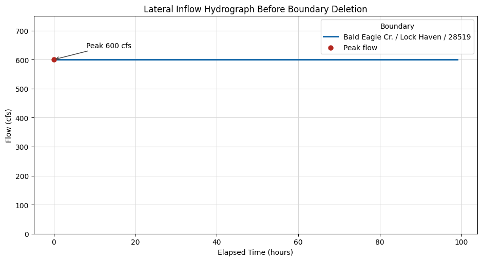
Non-Required Lateral Inflow Boundary Deletion

The CRUD delete operation should be demonstrated on an internal, non-required boundary. This section uses a separate copy of the official Dam Breaching example because it contains lateral inflow hydrographs in the unsteady flow file. The main Muncie workflow remains initialized in the global ras object; this delete demo uses its own RasPrj instance so it does not disturb the rest of the notebook.

Python

# Extract and initialize a separate project that has lateral inflow boundaries
delete_project_name = "Dam Breaching"
delete_project_path = RasExamples.extract_project(delete_project_name, suffix="300_delete_boundary")
delete_ras = RasPrj()
with temporary_logger_level("ras_commander.RasPrj", logging.ERROR):
    delete_ras.initialize(delete_project_path, RAS_VERSION, suppress_logging=True)

delete_unsteady_file = Path(
    delete_ras.unsteady_df.loc[delete_ras.unsteady_df["unsteady_number"] == "01", "full_path"].iloc[0]
)

boundaries_before_delete = delete_ras.boundaries_df.copy()
lateral_before = boundaries_before_delete[
    (boundaries_before_delete["unsteady_number"] == "01")
    & (boundaries_before_delete["bc_type"] == "Lateral Inflow Hydrograph")
].copy()

if lateral_before.empty:
    raise RuntimeError("Expected at least one lateral inflow boundary in the Dam Breaching example")

print(f"Delete demo project: {delete_project_path}")
print(f"Unsteady flow file: {delete_unsteady_file}")
print(f"Lateral inflow boundaries before delete: {len(lateral_before)}")

display_cols = [
    "unsteady_number",
    "boundary_condition_number",
    "bc_type",
    "river_reach_name",
    "river_station",
    "storage_area_name",
]
display(lateral_before[[c for c in display_cols if c in lateral_before.columns]])

Text Only

2026-06-03 15:12:39 - ras_commander.RasExamples - INFO - Successfully extracted project 'Dam Breaching' to C:\GH\symphony-workspaces\ras-commander\CLB-888\examples\example_projects\Dam Breaching_300_delete_boundary


2026-06-03 15:12:39 - ras_commander.RasMap - INFO - Successfully parsed RASMapper file: C:\GH\symphony-workspaces\ras-commander\CLB-888\examples\example_projects\Dam Breaching_300_delete_boundary\BaldEagleDamBrk.rasmap


Delete demo project: C:\GH\symphony-workspaces\ras-commander\CLB-888\examples\example_projects\Dam Breaching_300_delete_boundary
Unsteady flow file: C:\GH\symphony-workspaces\ras-commander\CLB-888\examples\example_projects\Dam Breaching_300_delete_boundary\BaldEagleDamBrk.u01
Lateral inflow boundaries before delete: 4

	unsteady_number	boundary_condition_number	bc_type	river_reach_name	river_station	storage_area_name
12	01	3	Lateral Inflow Hydrograph	Bald Eagle Cr.	Lock Haven	28519
13	01	4	Lateral Inflow Hydrograph	Bald Eagle Cr.	Lock Haven	1
14	01	5	Lateral Inflow Hydrograph	Bald Eagle Cr.	Lock Haven	76865
15	01	6	Lateral Inflow Hydrograph	Bald Eagle Cr.	Lock Haven	67130

Python

# Read and plot the lateral inflow hydrograph before deletion
target_boundary = lateral_before.iloc[0]
target_boundary_index = int(target_boundary["boundary_condition_number"]) - 1

delete_demo_bytes_before = delete_unsteady_file.read_bytes()
delete_demo_text_before = delete_demo_bytes_before.decode("utf-8", errors="ignore")

location_line = None
for line in delete_demo_text_before.splitlines():
    if line.startswith("Boundary Location="):
        loc_value = line[len("Boundary Location="):].rstrip("\r\n")
        parts = [part.strip() for part in loc_value.split(",")]
        if len(parts) >= 3 and parts[0] == target_boundary["river_reach_name"] and parts[2] == target_boundary["storage_area_name"]:
            location_line = line
            target_location_parts = parts
            break

if location_line is None:
    raise RuntimeError("Could not match the lateral inflow Boundary Location line")

target_river, target_reach, target_station = target_location_parts[:3]
target_header = f"Boundary Location={location_line[len('Boundary Location=') :]}"

lateral_hydrograph = RasUnsteady.get_lateral_inflow_hydrograph(
    delete_unsteady_file,
    river=target_river,
    reach=target_reach,
    station=target_station,
    ras_object=delete_ras,
)

if lateral_hydrograph is None or lateral_hydrograph.empty:
    raise RuntimeError("Could not read the target lateral inflow hydrograph")

interval_text = str(lateral_hydrograph.attrs.get("interval") or "1HOUR").upper()
interval_hours = 1.0
if "MIN" in interval_text:
    interval_hours = float("".join(ch for ch in interval_text if ch.isdigit() or ch == ".")) / 60.0
elif "HOUR" in interval_text:
    interval_hours = float("".join(ch for ch in interval_text if ch.isdigit() or ch == "."))

time_hours = np.arange(len(lateral_hydrograph)) * interval_hours
flows = lateral_hydrograph["flow"].to_numpy(dtype=float)
peak_idx = int(np.argmax(flows))
peak_hour = float(time_hours[peak_idx])
peak_flow = float(flows[peak_idx])

fig, ax = plt.subplots(figsize=(9.5, 5.2))
ax.plot(time_hours, flows, color="#1769aa", linewidth=2.2, label=f"{target_river} / {target_reach} / {target_station}")
ax.scatter([peak_hour], [peak_flow], color="#b3261e", s=42, zorder=3, label="Peak flow")
ax.annotate(
    f"Peak {peak_flow:,.0f} cfs",
    xy=(peak_hour, peak_flow),
    xytext=(peak_hour + max(time_hours.max() * 0.08, 4.0), peak_flow * 1.08),
    arrowprops={"arrowstyle": "->", "color": "#444444", "lw": 1.1},
    va="center",
)
ax.set_title("Lateral Inflow Hydrograph Before Boundary Deletion")
ax.set_xlabel("Elapsed Time (hours)")
ax.set_ylabel("Flow (cfs)")
ax.set_ylim(0, max(peak_flow * 1.25, 1.0))
ax.grid(True, color="#d7d7d7", linewidth=0.8)
ax.legend(title="Boundary", loc="best")
fig.tight_layout()
plt.show()

Text Only

2026-06-03 15:12:39 - ras_commander.RasUnsteady - INFO - Read Lateral Inflow Hydrograph from BaldEagleDamBrk.u01: 100 values, peak=600.0, interval=1HOUR, slope=None

Python

# Delete only the non-required lateral inflow Boundary Location block
delete_result = RasUnsteady.delete_boundary(
    delete_unsteady_file,
    river=target_river,
    reach=target_reach,
    river_station=target_station,
    boundary_index=target_boundary_index,
    ras_object=delete_ras,
)

print("Delete result:")
display(pd.DataFrame([delete_result]))

Text Only

2026-06-03 15:12:40 - ras_commander.RasUnsteady - INFO - Deleted boundary Bald Eagle Cr./Lock Haven/28519 (Lateral Inflow Hydrograph) from BaldEagleDamBrk.u01: 21 lines removed


Delete result:

	unsteady_file	deleted	name	matched_location	bc_type	boundary_index	backup_path	lines_removed	boundaries_df_refreshed	required_boundary
0	C:\GH\symphony-workspaces\ras-commander\CLB-88...	True	Bald Eagle Cr./Lock Haven/28519	Bald Eagle Cr.  ,Lock Haven      ,28519   ,   ...	Lateral Inflow Hydrograph	2	C:\GH\symphony-workspaces\ras-commander\CLB-88...	21	True	False

Python

# Re-read boundaries_df and confirm the block was removed and a .bak was written
boundaries_after_delete = delete_ras.boundaries_df.copy()
lateral_after = boundaries_after_delete[
    (boundaries_after_delete["unsteady_number"] == "01")
    & (boundaries_after_delete["bc_type"] == "Lateral Inflow Hydrograph")
].copy()

delete_demo_bytes_after = delete_unsteady_file.read_bytes()
delete_demo_text_after = delete_demo_bytes_after.decode("utf-8", errors="ignore")

backup_path = Path(delete_result["backup_path"])
checks = {
    "boundary_count_before": len(boundaries_before_delete),
    "boundary_count_after": len(boundaries_after_delete),
    "lateral_count_before_u01": len(lateral_before),
    "lateral_count_after_u01": len(lateral_after),
    "target_header_present_before": target_header in delete_demo_text_before,
    "target_header_present_after": target_header in delete_demo_text_after,
    "backup_exists": backup_path.exists(),
    "backup_matches_pre_delete_file": backup_path.read_bytes() == delete_demo_bytes_before,
}

for key, value in checks.items():
    print(f"{key}: {value}")

assert checks["target_header_present_before"] is True
assert checks["target_header_present_after"] is False
assert checks["backup_exists"] is True
assert checks["backup_matches_pre_delete_file"] is True
assert checks["boundary_count_after"] == checks["boundary_count_before"] - 1
assert checks["lateral_count_after_u01"] == checks["lateral_count_before_u01"] - 1

display(lateral_after[[c for c in display_cols if c in lateral_after.columns]])

Text Only

boundary_count_before: 36
boundary_count_after: 35
lateral_count_before_u01: 4
lateral_count_after_u01: 3
target_header_present_before: True
target_header_present_after: False
backup_exists: True
backup_matches_pre_delete_file: True

	unsteady_number	boundary_condition_number	bc_type	river_reach_name	river_station	storage_area_name
12	01	3	Lateral Inflow Hydrograph	Bald Eagle Cr.	Lock Haven	1
13	01	4	Lateral Inflow Hydrograph	Bald Eagle Cr.	Lock Haven	76865
14	01	5	Lateral Inflow Hydrograph	Bald Eagle Cr.	Lock Haven	67130

Python

# Confirm the post-delete project still initializes through ras-commander
post_delete_ras = RasPrj()
with temporary_logger_level("ras_commander.RasPrj", logging.ERROR):
    post_delete_ras.initialize(delete_project_path, RAS_VERSION, suppress_logging=True)
print(f"Post-delete initialization succeeded: {len(post_delete_ras.boundaries_df)} boundaries parsed")

Text Only

2026-06-03 15:12:40 - ras_commander.RasMap - INFO - Successfully parsed RASMapper file: C:\GH\symphony-workspaces\ras-commander\CLB-888\examples\example_projects\Dam Breaching_300_delete_boundary\BaldEagleDamBrk.rasmap


Post-delete initialization succeeded: 35 boundaries parsed

Step 4: Update Flow Title

The flow title in an unsteady flow file provides a description of the simulation scenario. The update_flow_title() method allows us to modify this title.

Parameters for RasUnsteady.update_flow_title(): - unsteady_file (str): Full path to the unsteady flow file - new_title (str): New flow title (max 24 characters) - ras_object (optional): Custom RAS object to use instead of the global one

Let's clone an unsteady flow file and update its title:

Python

# Clone unsteady flow "01" to create a new unsteady flow file
new_unsteady_number = RasPlan.clone_unsteady("01")
print(f"New unsteady flow created: {new_unsteady_number}")

Text Only

2026-06-03 15:12:40 - ras_commander.RasUtils - INFO - File cloned from C:\GH\symphony-workspaces\ras-commander\CLB-888\examples\example_projects\Muncie_300\Muncie.u01 to C:\GH\symphony-workspaces\ras-commander\CLB-888\examples\example_projects\Muncie_300\Muncie.u02


2026-06-03 15:12:40 - ras_commander.RasUtils - INFO - Project file updated with new Unsteady entry: 02


2026-06-03 15:12:40 - ras_commander.RasMap - INFO - Successfully parsed RASMapper file: C:\GH\symphony-workspaces\ras-commander\CLB-888\examples\example_projects\Muncie_300\Muncie.rasmap


New unsteady flow created: 02

Python

new_unsteady_number

Text Only

'02'

Python

# Get the path to the new unsteady flow file
new_unsteady_file = RasPlan.get_unsteady_path(new_unsteady_number)
print(f"New unsteady flow file path: {new_unsteady_file}")

Text Only

New unsteady flow file path: C:\GH\symphony-workspaces\ras-commander\CLB-888\examples\example_projects\Muncie_300\Muncie.u02

Python

new_unsteady_file

Text Only

WindowsPath('C:/GH/symphony-workspaces/ras-commander/CLB-888/examples/example_projects/Muncie_300/Muncie.u02')

Python

# Get the current flow title
current_title = None
for _, row in ras.unsteady_df.iterrows():
    if row['unsteady_number'] == new_unsteady_number and 'Flow Title' in row:
        current_title = row['Flow Title']
        break
print(f"Current flow title: {current_title}")

# Update the flow title
new_title = "Modified Flow Scenario"
RasUnsteady.update_flow_title(new_unsteady_file, new_title)
print(f"Updated flow title to: {new_title}")

# Refresh unsteady flow information to see the change

Text Only

2026-06-03 15:12:40 - ras_commander.RasUnsteady - INFO - Updated Flow Title from 'Flow Boundary Conditions' to 'Modified Flow Scenario'


2026-06-03 15:12:40 - ras_commander.RasUnsteady - INFO - Applied Flow Title modification to C:\GH\symphony-workspaces\ras-commander\CLB-888\examples\example_projects\Muncie_300\Muncie.u02


Current flow title: Flow Boundary Conditions
Updated flow title to: Modified Flow Scenario

Python

# Review unsteady flow information to see the change
ras.unsteady_df

	unsteady_number	full_path	Flow Title	Program Version	Use Restart	Restart Filename	Precipitation Mode	Wind Mode	Met BC=Precipitation|Expanded View	Met BC=Precipitation|Gridded Source	description
0	01	C:\GH\symphony-workspaces\ras-commander\CLB-88...	Flow Boundary Conditions	6.30	0	Muncie.p05.02JAN1900 1200.rst	Disable	No Wind Forces	0	DSS
1	02	C:\GH\symphony-workspaces\ras-commander\CLB-88...	Modified Flow Scenario	6.30	0	Muncie.p05.02JAN1900 1200.rst	Disable	No Wind Forces	0	DSS

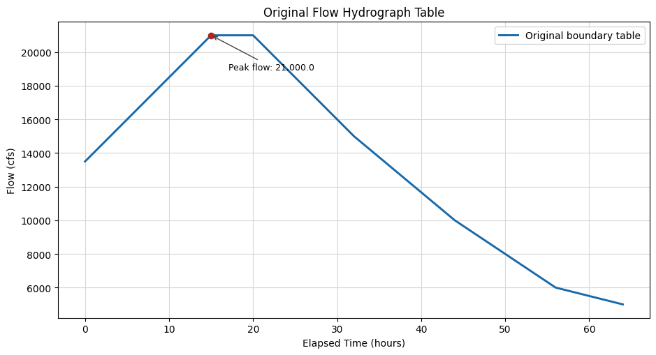
Step 6: Working with Flow Tables

Flow tables in unsteady flow files contain the time-series data for boundary conditions. Let's explore how to extract and work with these tables using some of the advanced methods from the RasUnsteady class.

Python

# Extract specific tables from the unsteady flow file
all_tables = RasUnsteady.extract_tables(new_unsteady_file)
print(f"Extracted {len(all_tables)} tables from the unsteady flow file.")

# Let's look at the available table names
print("\nAvailable tables:")
for table_name in all_tables.keys():
    print(f"  {table_name}")

# Select the first table for detailed analysis
if all_tables and len(all_tables) > 0:
    first_table_name = list(all_tables.keys())[0]
    first_table = all_tables[first_table_name]

    print(f"\nDetailed look at table '{first_table_name}':")
    print(f"  Number of values: {len(first_table)}")
    print(f"  Min value: {first_table['Value'].min()}")
    print(f"  Max value: {first_table['Value'].max()}")
    print(f"  Mean value: {first_table['Value'].mean():.2f}")
    print(f"  First 10 values: {first_table['Value'].head(10).tolist()}")

    # Create a technical hydrograph figure with explicit units.
    try:
        time_hours = np.arange(len(first_table), dtype=float)
        values = first_table['Value'].to_numpy(dtype=float)
        fig, ax = plt.subplots(figsize=(9.5, 5.2))
        ax.plot(time_hours, values, color="#1769aa", linewidth=2.1, label="Original boundary table")
        annotate_peak(ax, time_hours, values, label="Peak flow")
        ax.set_title("Original Flow Hydrograph Table")
        ax.set_xlabel("Elapsed Time (hours)")
        ax.set_ylabel("Flow (cfs)")
        ax.grid(True, color="#d7d7d7", linewidth=0.8)
        ax.legend(loc="best")
        fig.tight_layout()
        plt.show()
    except Exception as e:
        print(f"Could not create visualization: {e}")
else:
    print("No tables found in the unsteady flow file.")

Text Only

Extracted 1 tables from the unsteady flow file.

Available tables:
  Flow Hydrograph=

Detailed look at table 'Flow Hydrograph=':
  Number of values: 65
  Min value: 5000.0
  Max value: 21000.0
  Mean value: 13523.08
  First 10 values: [13500.0, 14000.0, 14500.0, 15000.0, 15500.0, 16000.0, 16500.0, 17000.0, 17500.0, 18000.0]

Step 7: Modifying Flow Tables

Now let's demonstrate how to modify a flow table and write it back to the unsteady flow file. For this example, we'll scale all the values in a table by a factor.

Scaling existing values down by a 0.75 scale factor

Python

# First, identify tables in the unsteady flow file
tables = RasUnsteady.identify_tables(open(new_unsteady_file, 'r').readlines())
print(f"Identified {len(tables)} tables in the unsteady flow file.")

# Let's look at the first flow hydrograph table
flow_hydrograph_tables = [t for t in tables if t[0] == 'Flow Hydrograph=']
if flow_hydrograph_tables:
    table_name, start_line, end_line = flow_hydrograph_tables[0]
    print(f"\nSelected table: {table_name}")
    print(f"  Start line: {start_line}")
    print(f"  End line: {end_line}")

    # Parse the table
    lines = open(new_unsteady_file, 'r').readlines()
    table_df = RasUnsteady.parse_fixed_width_table(lines, start_line, end_line)
    print(f"\nOriginal table statistics:")
    print(f"  Number of values: {len(table_df)}")
    print(f"  Min value: {table_df['Value'].min()}")
    print(f"  Max value: {table_df['Value'].max()}")
    print(f"  First 5 values: {table_df['Value'].head(5).tolist()}")

    # Modify the table - let's scale all values by 75%
    scale_factor = 0.75
    table_df['Value'] = table_df['Value'] * scale_factor
    print(f"\nModified table statistics (scaled by {scale_factor}):")
    print(f"  Number of values: {len(table_df)}")
    print(f"  Min value: {table_df['Value'].min()}")
    print(f"  Max value: {table_df['Value'].max()}")
    print(f"  First 5 values: {table_df['Value'].head(5).tolist()}")

    # Write the modified table back to the file
    RasUnsteady.write_table_to_file(new_unsteady_file, table_name, table_df, start_line)
    print(f"\nUpdated table written back to the unsteady flow file.")

    # Re-read the table to verify changes
    lines = open(new_unsteady_file, 'r').readlines()
    updated_table_df = RasUnsteady.parse_fixed_width_table(lines, start_line, end_line)
    print(f"\nVerified updated table statistics:")
    print(f"  Number of values: {len(updated_table_df)}")
    print(f"  Min value: {updated_table_df['Value'].min()}")
    print(f"  Max value: {updated_table_df['Value'].max()}")
    print(f"  First 5 values: {updated_table_df['Value'].head(5).tolist()}")
else:
    print("No flow hydrograph tables found in the unsteady flow file.")

Text Only

2026-06-03 15:12:40 - ras_commander.RasUnsteady - INFO - Successfully updated table 'Flow Hydrograph=' in C:\GH\symphony-workspaces\ras-commander\CLB-888\examples\example_projects\Muncie_300\Muncie.u02


Identified 1 tables in the unsteady flow file.

Selected table: Flow Hydrograph=
  Start line: 8
  End line: 15

Original table statistics:
  Number of values: 65
  Min value: 5000.0
  Max value: 21000.0
  First 5 values: [13500.0, 14000.0, 14500.0, 15000.0, 15500.0]

Modified table statistics (scaled by 0.75):
  Number of values: 65
  Min value: 3750.0
  Max value: 15750.0
  First 5 values: [10125.0, 10500.0, 10875.0, 11250.0, 11625.0]

Updated table written back to the unsteady flow file.

Verified updated table statistics:
  Number of values: 65
  Min value: 3750.0
  Max value: 15750.0
  First 5 values: [10125.0, 10500.0, 10875.0, 11250.0, 11625.0]

Python

# Extract specific tables from the unsteady flow file
all_tables = RasUnsteady.extract_tables(new_unsteady_file)

# Get the updated flow hydrograph table
flow_hydrograph_tables = [t for t in all_tables.keys() if 'Flow Hydrograph=' in t]
if flow_hydrograph_tables:
    table_name = flow_hydrograph_tables[0]
    table_df = all_tables[table_name]

    # Create visualization of the updated flow values
    time_hours = np.arange(len(table_df), dtype=float)
    values = table_df['Value'].to_numpy(dtype=float)
    fig, ax = plt.subplots(figsize=(9.5, 5.2))
    ax.plot(time_hours, values, color="#1769aa", linewidth=2.1, label="Updated flow")
    annotate_peak(ax, time_hours, values, label="Peak flow")
    ax.set_title("Updated Flow Hydrograph After 0.75 Scale Factor")
    ax.set_xlabel("Elapsed Time (hours)")
    ax.set_ylabel("Flow (cfs)")
    ax.grid(True, color="#d7d7d7", linewidth=0.8)
    ax.legend(loc="best")
    fig.tight_layout()
    plt.show()

    # Print summary statistics
    print(f"\nUpdated flow hydrograph statistics:")
    print(f"  Number of values: {len(table_df)}")
    print(f"  Min flow: {table_df['Value'].min():.1f} cfs")
    print(f"  Max flow: {table_df['Value'].max():.1f} cfs")
    print(f"  Mean flow: {table_df['Value'].mean():.1f} cfs")
else:
    print("No flow hydrograph tables found in the unsteady flow file.")

Text Only

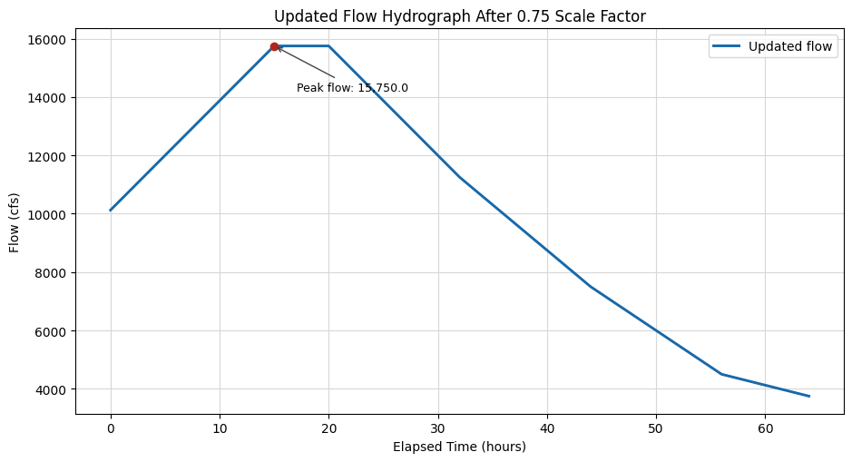
Updated flow hydrograph statistics:
  Number of values: 65
  Min flow: 3750.0 cfs
  Max flow: 15750.0 cfs
  Mean flow: 10142.3 cfs

Python

# Execute Plan 01 to generate model results

RasCmdr.compute_plan("01")

Text Only

2026-06-03 15:12:40 - ras_commander.RasCmdr - INFO - Using ras_object with project folder: C:\GH\symphony-workspaces\ras-commander\CLB-888\examples\example_projects\Muncie_300


2026-06-03 15:12:40 - ras_commander.RasCmdr - INFO - Running HEC-RAS from the Command Line:


2026-06-03 15:12:40 - ras_commander.RasCmdr - INFO - Running command: "C:\Program Files (x86)\HEC\HEC-RAS\7.0\Ras.exe" -c "C:\GH\symphony-workspaces\ras-commander\CLB-888\examples\example_projects\Muncie_300\Muncie.prj" "C:\GH\symphony-workspaces\ras-commander\CLB-888\examples\example_projects\Muncie_300\Muncie.p01"


2026-06-03 15:12:40 - ras_commander.RasDialogWatchdog - INFO - DialogWatchdog started — polling every 1.5s for RAS dialog windows


2026-06-03 15:12:53 - ras_commander.RasCmdr - INFO - HEC-RAS execution completed for plan: 01


2026-06-03 15:12:53 - ras_commander.RasCmdr - INFO - Total run time for plan 01: 12.82 seconds


2026-06-03 15:12:53 - ras_commander.RasDialogWatchdog - INFO - DialogWatchdog stopped — no dialogs encountered





ComputeResult(SUCCESS, results_df_row=available)

Python

# Display results summary from results_df after Plan 01 execution
# This shows execution status, timing, and any errors/warnings for each plan
ras.results_df[['plan_number', 'plan_title', 'completed', 'has_errors', 'has_warnings', 'runtime_complete_process_hours']]

	plan_number	plan_title	completed	has_errors	has_warnings	runtime_complete_process_hours
0	03	Unsteady Run with 2D 50ft Grid	False	False	False	NaN
1	04	Unsteady Run with 2D 50ft User n Value R	False	False	False	NaN
2	01	Unsteady Multi  9-SA run	True	False	False	0.003182

Python

# Get cross section results timeseries as xarray dataset
xsec_results_xr_plan1 = HdfResultsXsec.get_xsec_timeseries("01")

Python

xsec_results_xr_plan1

<xarray.Dataset> Size: 371kB
Dimensions:                   (time: 289, cross_section: 61)
Coordinates:
  * time                      (time) datetime64[us] 2kB 1900-01-02 ... 1900-0...
  * cross_section             (cross_section) <U42 10kB 'White            Mun...
    River                     (cross_section) <U5 1kB 'White' ... 'White'
    Reach                     (cross_section) <U6 1kB 'Muncie' ... 'Muncie'
    Station                   (cross_section) <U8 2kB '15696.24' ... '237.6455'
    Name                      (cross_section) <U1 244B '' '' '' '' ... '' '' ''
    Maximum_Water_Surface     (cross_section) float32 244B 955.4 955.2 ... 938.7
    Maximum_Flow              (cross_section) float32 244B 2.1e+04 ... 2.1e+04
    Maximum_Channel_Velocity  (cross_section) float32 244B 5.293 6.224 ... 6.081
    Maximum_Velocity_Total    (cross_section) float32 244B 3.472 4.026 ... 5.999
    Maximum_Flow_Lateral      (cross_section) float32 244B 0.0 0.0 ... 0.0 0.0
Data variables:
    Water_Surface             (time, cross_section) float32 71kB 951.4 ... 937.9
    Velocity_Total            (time, cross_section) float32 71kB 3.472 ... 5.909
    Velocity_Channel          (time, cross_section) float32 71kB 5.293 ... 5.934
    Flow_Lateral              (time, cross_section) float32 71kB 0.0 0.0 ... 0.0
    Flow                      (time, cross_section) float32 71kB 1.35e+04 ......
Attributes:
    description:  Cross-section results extracted from HEC-RAS HDF file
    source_file:  C:\GH\symphony-workspaces\ras-commander\CLB-888\examples\ex...

xarray.Dataset

• Dimensions:
  • time: 289
  • cross_section: 61
• Coordinates: (11)
  • time
    (time)
    datetime64[us]
    1900-01-02 ... 1900-01-03

    array(['1900-01-02T00:00:00.000000', '1900-01-02T00:05:00.000000',
           '1900-01-02T00:10:00.000000', ..., '1900-01-02T23:50:00.000000',
           '1900-01-02T23:55:00.000000', '1900-01-03T00:00:00.000000'],
          shape=(289,), dtype='datetime64[us]')

  • cross_section
    (cross_section)
    <U42
    'White Muncie ...

    array(['White            Muncie           15696.24',
           'White            Muncie           15485.51',
           'White            Muncie           15370.43',
           'White            Muncie           15205.29',
           'White            Muncie           15013.20',
           'White            Muncie           14917.36',
           'White            Muncie           14856.24',
           'White            Muncie           14787.40',
           'White            Muncie           14697.22',
           'White            Muncie           14535.60',
           'White            Muncie           14443.72',
           'White            Muncie           14305.48',
           'White            Muncie           14166.05',
           'White            Muncie           14039.64',
           'White            Muncie           13859.04',
           'White            Muncie           13490.47',
           'White            Muncie           13214.80',
           'White            Muncie           12817.36',
           'White            Muncie           12492.03',
           'White            Muncie           12227.69',
           'White            Muncie           12117.14',
           'White            Muncie           11958.11',
           'White            Muncie           11781.69',
           'White            Muncie           11628.65',
           'White            Muncie           11377.89',
           'White            Muncie           11188.16',
           'White            Muncie           10672.75',
           'White            Muncie           10216.27',
           'White            Muncie           9854.381',
           'White            Muncie           9548.851',
           'White            Muncie           9334.877',
           'White            Muncie           9081.195',
           'White            Muncie           8757.405',
           'White            Muncie           8434.332',
           'White            Muncie           8110.505',
           'White            Muncie           7864.487',
           'White            Muncie           7490.833',
           'White            Muncie           7158.903',
           'White            Muncie           6868.344',
           'White            Muncie           6626.553',
           'White            Muncie           6295.048',
           'White            Muncie           5925.654',
           'White            Muncie           5688.906',
           'White            Muncie           5382.517',
           'White            Muncie           5124.979',
           'White            Muncie           4850.811',
           'White            Muncie           4570.628',
           'White            Muncie           4185.719',
           'White            Muncie           3952.406',
           'White            Muncie           3690.809',
           'White            Muncie           3268.276',
           'White            Muncie           2920.440',
           'White            Muncie           2582.948',
           'White            Muncie           2290.221',
           'White            Muncie           1980.776',
           'White            Muncie           1743.103',
           'White            Muncie           1469.294',
           'White            Muncie           1174.213',
           'White            Muncie           865.5413',
           'White            Muncie           570.1187',
           'White            Muncie           237.6455'], dtype='<U42')

  • River
    (cross_section)
    <U5
    'White' 'White' ... 'White' 'White'

    array(['White', 'White', 'White', 'White', 'White', 'White', 'White',
           'White', 'White', 'White', 'White', 'White', 'White', 'White',
           'White', 'White', 'White', 'White', 'White', 'White', 'White',
           'White', 'White', 'White', 'White', 'White', 'White', 'White',
           'White', 'White', 'White', 'White', 'White', 'White', 'White',
           'White', 'White', 'White', 'White', 'White', 'White', 'White',
           'White', 'White', 'White', 'White', 'White', 'White', 'White',
           'White', 'White', 'White', 'White', 'White', 'White', 'White',
           'White', 'White', 'White', 'White', 'White'], dtype='<U5')

  • Reach
    (cross_section)
    <U6
    'Muncie' 'Muncie' ... 'Muncie'

    array(['Muncie', 'Muncie', 'Muncie', 'Muncie', 'Muncie', 'Muncie',
           'Muncie', 'Muncie', 'Muncie', 'Muncie', 'Muncie', 'Muncie',
           'Muncie', 'Muncie', 'Muncie', 'Muncie', 'Muncie', 'Muncie',
           'Muncie', 'Muncie', 'Muncie', 'Muncie', 'Muncie', 'Muncie',
           'Muncie', 'Muncie', 'Muncie', 'Muncie', 'Muncie', 'Muncie',
           'Muncie', 'Muncie', 'Muncie', 'Muncie', 'Muncie', 'Muncie',
           'Muncie', 'Muncie', 'Muncie', 'Muncie', 'Muncie', 'Muncie',
           'Muncie', 'Muncie', 'Muncie', 'Muncie', 'Muncie', 'Muncie',
           'Muncie', 'Muncie', 'Muncie', 'Muncie', 'Muncie', 'Muncie',
           'Muncie', 'Muncie', 'Muncie', 'Muncie', 'Muncie', 'Muncie',
           'Muncie'], dtype='<U6')

  • Station
    (cross_section)
    <U8
    '15696.24' ... '237.6455'

    array(['15696.24', '15485.51', '15370.43', '15205.29', '15013.20',
           '14917.36', '14856.24', '14787.40', '14697.22', '14535.60',
           '14443.72', '14305.48', '14166.05', '14039.64', '13859.04',
           '13490.47', '13214.80', '12817.36', '12492.03', '12227.69',
           '12117.14', '11958.11', '11781.69', '11628.65', '11377.89',
           '11188.16', '10672.75', '10216.27', '9854.381', '9548.851',
           '9334.877', '9081.195', '8757.405', '8434.332', '8110.505',
           '7864.487', '7490.833', '7158.903', '6868.344', '6626.553',
           '6295.048', '5925.654', '5688.906', '5382.517', '5124.979',
           '4850.811', '4570.628', '4185.719', '3952.406', '3690.809',
           '3268.276', '2920.440', '2582.948', '2290.221', '1980.776',
           '1743.103', '1469.294', '1174.213', '865.5413', '570.1187',
           '237.6455'], dtype='<U8')

  • Name
    (cross_section)
    <U1
    '' '' '' '' '' ... '' '' '' '' ''

    array(['', '', '', '', '', '', '', '', '', '', '', '', '', '', '', '', '',
           '', '', '', '', '', '', '', '', '', '', '', '', '', '', '', '', '',
           '', '', '', '', '', '', '', '', '', '', '', '', '', '', '', '', '',
           '', '', '', '', '', '', '', '', '', ''], dtype='<U1')

  • Maximum_Water_Surface
    (cross_section)
    float32
    955.4 955.2 955.0 ... 939.1 938.7

    array([955.4193 , 955.174  , 954.9523 , 954.893  , 954.5605 , 953.98663,
           953.5865 , 953.6952 , 953.3395 , 953.2332 , 952.32056, 950.1069 ,
           950.79956, 947.9223 , 948.7183 , 948.813  , 948.6352 , 948.31995,
           948.2081 , 947.2089 , 946.9157 , 947.28906, 946.92126, 946.67676,
           946.15674, 946.20935, 945.87885, 945.4968 , 944.7825 , 944.87036,
           944.805  , 944.67914, 944.7106 , 944.65533, 944.5989 , 944.4735 ,
           944.05035, 943.9091 , 943.6594 , 943.8137 , 943.22705, 943.0823 ,
           942.6955 , 942.75684, 942.5032 , 942.21155, 941.9739 , 941.856  ,
           941.4769 , 941.1461 , 941.1205 , 940.90094, 940.4076 , 939.86304,
           939.7989 , 939.4432 , 939.4007 , 939.3928 , 939.1499 , 939.0609 ,
           938.72864], dtype=float32)

  • Maximum_Flow
    (cross_section)
    float32
    2.1e+04 2.1e+04 ... 2.1e+04 2.1e+04

    array([21000.   , 21000.098, 21000.08 , 21000.059, 21000.047, 21000.033,
           21000.057, 21000.047, 21000.03 , 21000.05 , 21000.031, 21000.229,
           21000.861, 21000.586, 21000.092, 21000.037, 21000.102, 21000.025,
           17900.125, 17892.715, 17890.504, 17885.465, 17878.643, 17873.438,
           17864.984, 17858.408, 17840.93 , 17823.75 , 17818.703, 17818.672,
           17818.654, 17818.691, 17818.617, 17818.314, 17818.523, 17818.209,
           17817.945, 17911.686, 18016.37 , 18067.895, 18088.84 , 18089.225,
           18095.703, 18122.78 , 18167.887, 18241.455, 18332.232, 18472.182,
           18572.732, 18685.682, 18907.916, 19246.691, 19660.053, 19997.605,
           20295.408, 20569.336, 20832.588, 20998.082, 20997.988, 20998.027,
           20997.979], dtype=float32)

  • Maximum_Channel_Velocity
    (cross_section)
    float32
    5.293 6.224 6.953 ... 5.193 6.081

    array([ 5.29273  ,  6.22362  ,  6.9527273,  6.396673 ,  6.670246 ,
            8.393395 ,  9.820168 ,  8.389862 ,  9.434381 ,  8.123526 ,
           10.904437 , 15.102488 , 10.429727 , 18.536852 ,  7.966175 ,
            3.6401148,  5.016905 ,  4.977982 ,  3.868829 ,  9.455522 ,
            8.959682 ,  4.437134 ,  6.7612996,  6.6352954,  7.9893017,
            5.4494414,  5.304875 ,  5.8271027,  9.99514  ,  6.172858 ,
            5.126846 ,  6.7661347,  5.5544477,  5.2234664,  4.415842 ,
            5.614221 ,  6.12938  ,  5.5774574,  6.292568 ,  4.159369 ,
            7.128479 ,  6.52268  ,  7.728083 ,  5.925791 ,  6.6601634,
            7.2057714,  7.1674647,  5.8894653,  7.725181 ,  8.617449 ,
            5.5148797,  5.6485405,  7.3631573,  8.8674345,  6.3818555,
           13.525607 ,  6.9899774,  4.453645 ,  5.6350284,  5.192719 ,
            6.080602 ], dtype=float32)

  • Maximum_Velocity_Total
    (cross_section)
    float32
    3.472 4.026 4.818 ... 5.073 5.999

    array([ 3.4716372,  4.026342 ,  4.817801 ,  4.3600926,  4.8718634,
            7.293384 ,  8.068419 ,  7.2434783,  7.7842197,  7.2513976,
            9.492176 , 13.360935 ,  8.952023 , 16.875135 ,  6.7580385,
            2.0472884,  3.3148298,  2.7198005,  2.4577897,  8.110415 ,
            7.727931 ,  3.460086 ,  5.474504 ,  5.5779634,  7.849447 ,
            5.1736593,  5.016009 ,  5.445335 ,  9.416697 ,  5.726774 ,
            4.9780583,  6.6343856,  5.0011473,  5.1404734,  4.4158382,
            5.614214 ,  5.6776156,  5.4570374,  5.909942 ,  4.020742 ,
            6.888995 ,  6.269651 ,  7.3961744,  5.707138 ,  6.464431 ,
            6.587439 ,  6.495528 ,  5.532432 ,  6.5907493,  7.0161405,
            4.9984236,  5.1398683,  6.2922688,  8.334925 ,  5.70317  ,
           11.930439 ,  6.989966 ,  4.050681 ,  4.8599486,  5.0728946,
            5.9992576], dtype=float32)

  • Maximum_Flow_Lateral
    (cross_section)
    float32
    0.0 0.0 0.0 0.0 ... 0.0 0.0 0.0 0.0

    array([  0.       ,   0.       ,   0.       ,   0.       ,   0.       ,
             0.       ,   0.       ,   0.       ,   0.       ,   0.       ,
             0.       ,   0.       ,   0.       ,   0.       ,   0.       ,
             0.       ,   0.       ,   0.       ,   0.       ,   0.       ,
             0.       ,   0.       ,   0.       ,   0.       ,   0.       ,
             0.       ,   0.       ,   0.       ,   0.       ,   0.       ,
             0.       ,   0.       ,   0.       ,   0.       ,   0.       ,
             0.       ,  93.740425 , 104.72848  ,  51.504364 ,  20.928728 ,
             0.4568774,   6.475466 ,  27.027529 ,  45.117245 ,  73.63606  ,
            90.87834  , 139.9611   , 100.52647  , 112.97791  , 222.25061  ,
           338.8145   , 413.41354  , 337.5985   , 297.72806  , 274.00183  ,
           263.3059   , 165.4183   ,   0.       ,   0.       ,   0.       ,
             0.       ], dtype=float32)

• Data variables: (5)
  • Water_Surface
    (time, cross_section)
    float32
    951.4 951.2 951.0 ... 938.3 937.9

    array([[951.4461 , 951.1977 , 950.9904 , ..., 920.6691 , 920.56696,
            920.37775],
           [952.6853 , 952.49445, 952.3294 , ..., 920.62506, 920.5244 ,
            920.33606],
           [952.97394, 952.78467, 952.6197 , ..., 920.5882 , 920.488  ,
            920.2998 ],
           ...,
           [954.7896 , 954.55493, 954.3441 , ..., 938.4081 , 938.318  ,
            937.9907 ],
           [954.77545, 954.5411 , 954.3305 , ..., 938.38574, 938.2956 ,
            937.9684 ],
           [954.7613 , 954.52716, 954.3168 , ..., 938.3614 , 938.271  ,
            937.94354]], shape=(289, 61), dtype=float32)

  • Velocity_Total
    (time, cross_section)
    float32
    3.472 3.797 4.453 ... 4.974 5.909

    array([[3.4716372, 3.7973714, 4.4530463, ..., 1.8250524, 1.8691283,
            2.2576067],
           [2.9427826, 3.3591197, 3.9799016, ..., 1.8015527, 1.8451436,
            2.2486742],
           [2.8470454, 3.3110573, 3.9499834, ..., 1.8023059, 1.8358164,
            2.2407656],
           ...,
           [3.252479 , 3.877704 , 4.6397724, ..., 4.762067 , 4.9775124,
            5.9113374],
           [3.250214 , 3.8744507, 4.6358647, ..., 4.759134 , 4.974428 ,
            5.908647 ],
           [3.247921 , 3.8711343, 4.6318865, ..., 4.7583222, 4.973939 ,
            5.9089894]], shape=(289, 61), dtype=float32)

  • Velocity_Channel
    (time, cross_section)
    float32
    5.293 5.777 6.297 ... 5.06 5.934

    array([[5.29273  , 5.776688 , 6.297461 , ..., 1.8250555, 1.8691316,
            2.2576118],
           [4.5389576, 5.138783 , 5.6741257, ..., 1.8015558, 1.8451468,
            2.2486792],
           [4.4022117, 5.0714874, 5.6404552, ..., 1.802309 , 1.8358197,
            2.2407706],
           ...,
           [5.0980244, 5.9787507, 6.67794  , ..., 5.4830866, 5.0652823,
            5.939163 ],
           [5.0938888, 5.9734206, 6.6719136, ..., 5.4784956, 5.0613866,
            5.934774 ],
           [5.0897126, 5.9679947, 6.6657877, ..., 5.476257 , 5.0600653,
            5.933672 ]], shape=(289, 61), dtype=float32)

  • Flow_Lateral
    (time, cross_section)
    float32
    0.0 0.0 0.0 0.0 ... 0.0 0.0 0.0 0.0

    array([[0., 0., 0., ..., 0., 0., 0.],
           [0., 0., 0., ..., 0., 0., 0.],
           [0., 0., 0., ..., 0., 0., 0.],
           ...,
           [0., 0., 0., ..., 0., 0., 0.],
           [0., 0., 0., ..., 0., 0., 0.],
           [0., 0., 0., ..., 0., 0., 0.]], shape=(289, 61), dtype=float32)

  • Flow
    (time, cross_section)
    float32
    1.35e+04 1.283e+04 ... 1.955e+04

    array([[13500.     , 12825.791  , 12489.289  , ...,  1039.2759 ,
             1040.4172 ,  1041.6    ],
           [13541.667  , 13313.447  , 13207.51   , ...,  1015.71265,
             1020.75714,  1026.1938 ],
           [13583.333  , 13563.229  , 13555.144  , ...,  1007.91864,
             1010.2389 ,  1012.82434],
           ...,
           [19083.334  , 19088.496  , 19090.773  , ..., 19608.818  ,
            19614.783  , 19621.143  ],
           [19041.666  , 19046.76   , 19049.014  , ..., 19567.78   ,
            19573.705  , 19579.99   ],
           [19000.     , 19005.168  , 19007.41   , ..., 19533.715  ,
            19540.857  , 19548.217  ]], shape=(289, 61), dtype=float32)

• Attributes: (2)

  description :

  Cross-section results extracted from HEC-RAS HDF file

  source_file :

  C:\GH\symphony-workspaces\ras-commander\CLB-888\examples\example_projects\Muncie_300\Muncie.p01.hdf

Python

# Print time series for specific cross section
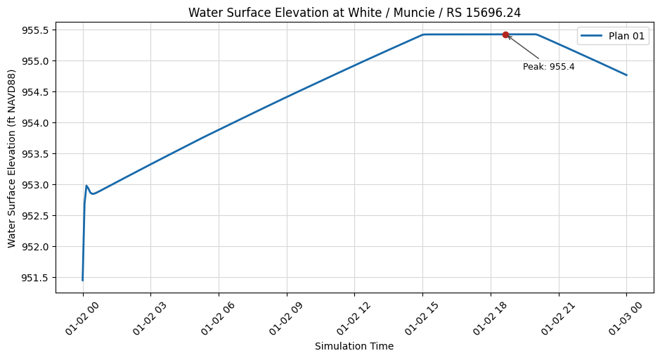
# Use a valid cross section from the Muncie project
target_xs = "White            Muncie           15696.24"
target_xs_label = "White / Muncie / RS 15696.24"

print("\nTime Series Data for Cross Section:", target_xs)
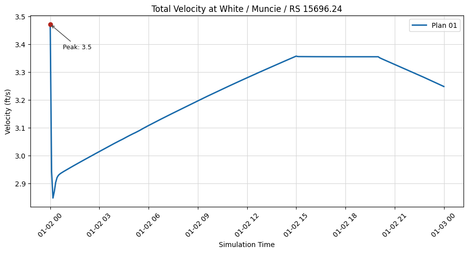
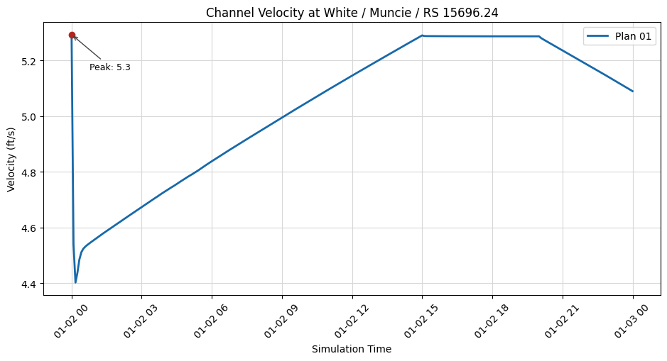
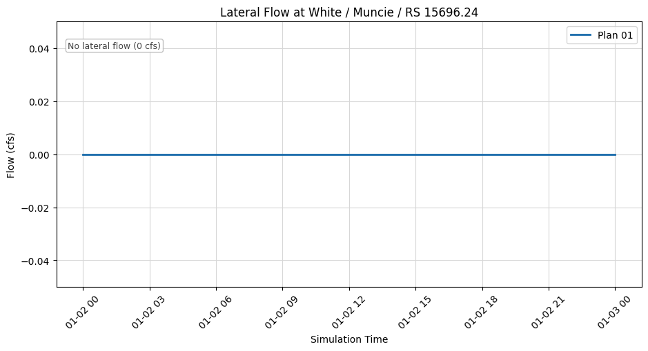
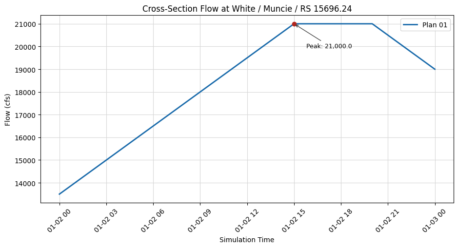
for var in ['Water_Surface', 'Velocity_Total', 'Velocity_Channel', 'Flow_Lateral', 'Flow']:
    print(f"\n{var}:")
    print(f"Plan 1:")
    print(xsec_results_xr_plan1[var].sel(cross_section=target_xs).values[:5])

# Create time series plots
if generate_plots:
    variables = ['Water_Surface', 'Velocity_Total', 'Velocity_Channel', 'Flow_Lateral', 'Flow']
    time_values1 = pd.to_datetime(xsec_results_xr_plan1.time.values)

    for var in variables:
        values1 = xsec_results_xr_plan1[var].sel(cross_section=target_xs).values
        labels = PLOT_LABELS.get(var, {"title": var.replace("_", " "), "ylabel": var.replace("_", " ")})

        fig, ax = plt.subplots(figsize=(9.5, 5.2))
        ax.plot(time_values1, values1, '-', linewidth=2, color="#1769aa", label='Plan 01')
        annotate_peak(ax, time_values1, values1, label="Peak")
        ax.set_title(f"{labels['title']} at {target_xs_label}")
        ax.set_xlabel('Simulation Time')
        ax.set_ylabel(labels['ylabel'])
        ax.grid(True, color="#d7d7d7", linewidth=0.8)
        ax.tick_params(axis='x', rotation=45)
        ax.legend(loc="best")
        fig.tight_layout()
        plt.show()

Text Only

Time Series Data for Cross Section: White            Muncie           15696.24

Water_Surface:
Plan 1:
[951.4461  952.6853  952.97394 952.9312  952.8653 ]

Velocity_Total:
Plan 1:
[3.4716372 2.9427826 2.8470454 2.8707995 2.9032633]

Velocity_Channel:
Plan 1:
[5.29273   4.5389576 4.4022117 4.437299  4.4849114]

Flow_Lateral:
Plan 1:
[0. 0. 0. 0. 0.]

Flow:
Plan 1:
[13500.    13541.667 13583.333 13625.    13666.667]

Step 8: Applying the Updated Unsteady Flow to a New Plan

Now that we've modified an unsteady flow file, let's create a plan that uses it, and compute the results.

Python

# Clone an existing plan
new_plan_number = RasPlan.clone_plan("01", new_plan_shortid="Modified Flow Test")
print(f"New plan created: {new_plan_number}")

Text Only

2026-06-03 15:12:54 - ras_commander.RasUtils - INFO - File cloned from C:\GH\symphony-workspaces\ras-commander\CLB-888\examples\example_projects\Muncie_300\Muncie.p01 to C:\GH\symphony-workspaces\ras-commander\CLB-888\examples\example_projects\Muncie_300\Muncie.p02


2026-06-03 15:12:54 - ras_commander.RasUtils - INFO - Successfully updated file: C:\GH\symphony-workspaces\ras-commander\CLB-888\examples\example_projects\Muncie_300\Muncie.p02


2026-06-03 15:12:54 - ras_commander.RasUtils - INFO - Project file updated with new Plan entry: 02


2026-06-03 15:12:54 - ras_commander.RasMap - INFO - Successfully parsed RASMapper file: C:\GH\symphony-workspaces\ras-commander\CLB-888\examples\example_projects\Muncie_300\Muncie.rasmap


New plan created: 02

Python

new_plan_number

Text Only

'02'

Python

# Get the current plan title and shortid
current_title = RasPlan.get_plan_title(new_plan_number)
current_shortid = RasPlan.get_shortid(new_plan_number)

print(f"Current plan title: {current_title}")
print(f"Current plan shortid: {current_shortid}")

Text Only

2026-06-03 15:12:54 - ras_commander.RasPlan - INFO - Retrieved Plan Title: Unsteady Multi  9-SA run


2026-06-03 15:12:54 - ras_commander.RasPlan - INFO - Retrieved Short Identifier: Modified Flow Test


Current plan title: Unsteady Multi  9-SA run
Current plan shortid: Modified Flow Test

Python

# Update the title and shortid to append "clonedplan"
new_title = f"{current_title} 0.75 Flow Scale Factor"
new_shortid = "Mod Flow 0.75 FSF"

RasPlan.set_plan_title(new_plan_number, new_title)
RasPlan.set_shortid(new_plan_number, new_shortid)

print()
print(f"Updated plan title: {RasPlan.get_plan_title(new_plan_number)}")
print(f"Updated plan shortid: {RasPlan.get_shortid(new_plan_number)}")

Text Only

2026-06-03 15:12:54 - ras_commander.RasPlan - INFO - Updated Plan Title in plan file to: Unsteady Multi  9-SA run 0.75 Flow Scale Factor


2026-06-03 15:12:54 - ras_commander.RasPlan - INFO - Updated Short Identifier in plan file to: Mod Flow 0.75 FSF


2026-06-03 15:12:54 - ras_commander.RasPlan - INFO - Retrieved Plan Title: Unsteady Multi  9-SA run 0.75 Flow Scale Factor


2026-06-03 15:12:54 - ras_commander.RasPlan - INFO - Retrieved Short Identifier: Mod Flow 0.75 FSF



Updated plan title: Unsteady Multi  9-SA run 0.75 Flow Scale Factor
Updated plan shortid: Mod Flow 0.75 FSF

Python

# Print new_unsteady_number again as a reminder of it's current value
new_unsteady_number

Text Only

'02'

Python

# Set the modified unsteady flow for the new plan
RasPlan.set_unsteady(new_plan_number, new_unsteady_number)
print(f"Set unsteady flow {new_unsteady_number} for plan {new_plan_number}")

Text Only

Set unsteady flow 02 for plan 02

Python

# Get the path to the new plan file
new_plan_path = RasPlan.get_plan_path(new_plan_number)

# Print contents of new plan file to confirm changes
# Read and display the contents of the plan file
with open(new_plan_path, 'r') as f:
    plan_contents = f.read()
print(f"Contents of plan file {new_plan_number}:")
print(plan_contents)

Text Only

Contents of plan file 02:
Plan Title=Unsteady Multi  9-SA run 0.75 Flow Scale Factor
Program Version=5.00
Short Identifier=Mod Flow 0.75 FSF
Simulation Date=02JAN1900,0000,02JAN1900,2400
Geom File=g01
Flow File=u02
Subcritical Flow
K Sum by GR= 0 
Std Step Tol= 0.01 
Critical Tol= 0.01 
Num of Std Step Trials= 20 
Max Error Tol= 0.3 
Flow Tol Ratio= 0.001 
Split Flow NTrial= 30 
Split Flow Tol= 0.02 
Split Flow Ratio= 0.02 
Log Output Level= 0 
Friction Slope Method= 1 
Unsteady Friction Slope Method= 2 
Unsteady Bridges Friction Slope Method= 1 
Parabolic Critical Depth
Global Vel Dist= 0 , 0 , 0 
Global Log Level= 0 
CheckData=True
Encroach Param=-1 ,0,0, 0 
Computation Interval=15SEC
Output Interval=5MIN
Run HTab= 1 
Run UNet= 1 
Run Sediment= 0 
Run PostProcess= 1 
Run WQNet= 0 
Run RASMapper= 0 
UNET Theta= 1 
UNET Theta Warmup= 1 
UNET ZTol= 0.02 
UNET ZSATol= 0.02 
UNET QTol=
UNET MxIter= 20 
UNET Max Iter WO Improvement= 0 
UNET MaxInSteps= 20 
UNET DtIC= 0 
UNET DtMin= 0 
UNET MaxCRTS= 20 
UNET WFStab= 2 
UNET SFStab= 1 
UNET WFX= 3 
UNET SFX= 1 
UNET DSS MLevel= 4 
UNET Pardiso=0
UNET DZMax Abort= 100 
UNET Use Existing IB Tables=-1 
UNET Froude Reduction=False
UNET Froude Limit= 1 
UNET Froude Power= 10 
UNET Time Slicing=0,0, 5 
UNET Junction Losses=0
UNET D1 Cores= 0 
UNET D2 Coriolis=-1
UNET D2 Cores= 0 
UNET D2 Theta= 1 
UNET D2 Theta Warmup= 1 
UNET D2 Z Tol= 0.01 
UNET D2 Max Iterations= 20 
UNET D2 Equation= 0 
UNET D2 TotalICTime=
UNET D2 RampUpFraction=0.5
UNET D2 TimeSlices= 1 
UNET D2 Eddy Viscosity=
UNET D2 BCVolumeCheck=0
UNET D2 Latitude=
UNET D1D2 MaxIter= 0 
UNET D1D2 ZTol=0.01
UNET D1D2 QTol=0.1
UNET D1D2 MinQTol=1
Instantaneous Interval=1HOUR
Mapping Interval=5MIN
DSS File=dss
Write IC File= 0 
Write IC File at Fixed DateTime=0
IC Time=,,
Write IC File Reoccurance=
Write IC File at Sim End=0
Echo Input=False
Echo Parameters=False
Echo Output=False
Write Detailed= 1 
HDF Write Warmup=0
HDF Write Time Slices=0
HDF Flush=0
HDF Compression= 1 
HDF Chunk Size= 1 
HDF Spatial Parts= 1 
HDF Use Max Rows=0
HDF Fixed Rows= 1 
Breach Loc=White           ,Muncie          ,13214   ,True,                
Breach Method= 0 
Breach Geom=600,100,942,0.2,0.2,True,0.5,945,2,2.6
Breach Start=True,947,,,False,,
Breach Progression= 2 
       0       0       1       1
Simplified Physical Breach Downcutting= 2 
       0       0       1       1
Simplified Physical Breach Widening= 2 
       0       0       1       1
Starting Notch Depth= 3.402823E+38 
Initial Piping Diameter= 3.402823E+38 
Mass Wasting Options= 0 
Mass Wasting Width= 3.402823E+38 
Mass Wasting Duration= 3.402823E+38 
Mass Wasting Final Bottom Elevation= 3.402823E+38 
Breach Use User Defined Growth Ratio=0
Breach User Defined Growth Ratio=1
Breach Loc=White           ,Muncie          ,7300    ,False,                
Breach Method= 0 
Breach Geom=,,,,,False,0.5,,,2.6
Breach Start=True,,,,False,,
Breach Progression= 2 
       0       0       1       1
Simplified Physical Breach Downcutting= 2 
       0       0       1       1
Simplified Physical Breach Widening= 2 
       0       0       1       1
Starting Notch Depth= 3.402823E+38 
Initial Piping Diameter= 3.402823E+38 
Mass Wasting Options= 0 
Mass Wasting Width= 3.402823E+38 
Mass Wasting Duration= 3.402823E+38 
Mass Wasting Final Bottom Elevation= 3.402823E+38 
Breach Use User Defined Growth Ratio=0
Breach User Defined Growth Ratio=1
Breach Loc=White           ,Muncie          ,12300   ,False,                
Breach Method= 0 
Breach Geom=,,,,,False,0.5,,,2.6
Breach Start=True,,,,False,,
Breach Progression= 2 
       0       0       1       1
Simplified Physical Breach Downcutting= 2 
       0       0       1       1
Simplified Physical Breach Widening= 2 
       0       0       1       1
Starting Notch Depth= 3.402823E+38 
Initial Piping Diameter= 3.402823E+38 
Mass Wasting Options= 0 
Mass Wasting Width= 3.402823E+38 
Mass Wasting Duration= 3.402823E+38 
Mass Wasting Final Bottom Elevation= 3.402823E+38 
Breach Use User Defined Growth Ratio=0
Breach User Defined Growth Ratio=1
Breach Loc=White           ,Muncie          ,9854    ,False,                
Breach Method= 0 
Breach Geom=,,,,,False,0.5,,,2.6
Breach Start=True,,,,False,,
Breach Progression= 2 
       0       0       1       1
Simplified Physical Breach Downcutting= 2 
       0       0       1       1
Simplified Physical Breach Widening= 2 
       0       0       1       1
Starting Notch Depth= 3.402823E+38 
Initial Piping Diameter= 3.402823E+38 
Mass Wasting Options= 0 
Mass Wasting Width= 3.402823E+38 
Mass Wasting Duration= 3.402823E+38 
Mass Wasting Final Bottom Elevation= 3.402823E+38 
Breach Use User Defined Growth Ratio=0
Breach User Defined Growth Ratio=1
Breach Loc=White           ,Muncie          ,9200    ,False,                
Breach Method= 0 
Breach Geom=,,,,,False,0.5,,,2.6
Breach Start=True,,,,False,,
Breach Progression= 2 
       0       0       1       1
Simplified Physical Breach Downcutting= 2 
       0       0       1       1
Simplified Physical Breach Widening= 2 
       0       0       1       1
Starting Notch Depth= 3.402823E+38 
Initial Piping Diameter= 3.402823E+38 
Mass Wasting Options= 0 
Mass Wasting Width= 3.402823E+38 
Mass Wasting Duration= 3.402823E+38 
Mass Wasting Final Bottom Elevation= 3.402823E+38 
Breach Use User Defined Growth Ratio=0
Breach User Defined Growth Ratio=1
Breach Loc=White           ,Muncie          ,8000    ,False,                
Breach Method= 0 
Breach Geom=,,,,,False,0.5,,,2.6
Breach Start=True,,,,False,,
Breach Progression= 2 
       0       0       1       1
Simplified Physical Breach Downcutting= 2 
       0       0       1       1
Simplified Physical Breach Widening= 2 
       0       0       1       1
Starting Notch Depth= 3.402823E+38 
Initial Piping Diameter= 3.402823E+38 
Mass Wasting Options= 0 
Mass Wasting Width= 3.402823E+38 
Mass Wasting Duration= 3.402823E+38 
Mass Wasting Final Bottom Elevation= 3.402823E+38 
Breach Use User Defined Growth Ratio=0
Breach User Defined Growth Ratio=1
Breach Loc=White           ,Muncie          ,15323.14,False,                
Breach Method= 0 
Breach Geom=,,,,,False,0.5,,,2.6
Breach Start=True,,,,False,,
Breach Progression= 2 
       0       0       1       1
Simplified Physical Breach Downcutting= 2 
       0       0       1       1
Simplified Physical Breach Widening= 2 
       0       0       1       1
Starting Notch Depth= 3.402823E+38 
Initial Piping Diameter= 3.402823E+38 
Mass Wasting Options= 0 
Mass Wasting Width= 3.402823E+38 
Mass Wasting Duration= 3.402823E+38 
Mass Wasting Final Bottom Elevation= 3.402823E+38 
Breach Use User Defined Growth Ratio=0
Breach User Defined Growth Ratio=1
Breach Loc=White           ,Muncie          ,13859   ,False,                
Breach Method= 0 
Breach Geom=,,,,,False,0.5,,,2.6
Breach Start=True,,,,False,,
Breach Progression= 2 
       0       0       1       1
Simplified Physical Breach Downcutting= 2 
       0       0       1       1
Simplified Physical Breach Widening= 2 
       0       0       1       1
Starting Notch Depth= 3.402823E+38 
Initial Piping Diameter= 3.402823E+38 
Mass Wasting Options= 0 
Mass Wasting Width= 3.402823E+38 
Mass Wasting Duration= 3.402823E+38 
Mass Wasting Final Bottom Elevation= 3.402823E+38 
Breach Use User Defined Growth Ratio=0
Breach User Defined Growth Ratio=1
Calibration Method= 0 
Calibration Iterations= 100 
Calibration Max Change=0.05
Calibration Tolerance=0.01
Calibration Maximum=1.5
Calibration Minimum=0.5
Calibration Optimization Method= 0 
Calibration Window=,,,
WQ AD Non Conservative
WQ ULTIMATE=-1
WQ Max Comp Step=1HOUR
WQ Output Interval=15MIN
WQ Output Selected Increments= 0 
WQ Output face flow=0
WQ Output face velocity=0
WQ Output face area=0
WQ Output face dispersion=0
WQ Output cell volume=0
WQ Output cell surface area=0
WQ Output cell continuity=0
WQ Output cumulative cell continuity=0
WQ Output face conc=0
WQ Output face dconc_dx=0
WQ Output face courant=0
WQ Output face peclet=0
WQ Output face adv mass=0
WQ Output face disp mass=0
WQ Output cell mass=0
WQ Output cell source sink temp=0
WQ Output nsm pathways=0
WQ Output nsm derived pathways=0
WQ Output MaxMinRange=-1
WQ Daily Max Min Mean=-1
WQ Daily Range=0
WQ Daily Time=0
WQ Create Restart=0
WQ Fixed Restart=0
WQ Restart Simtime=
WQ Restart Date=
WQ Restart Hour=
WQ System Summary=0
WQ Write To DSS=0
WQ Use Fixed Temperature=0
WQ Fixed Temperature=
Sorting and Armoring Iterations= 10 
XS Update Threshold= 0.02 
Bed Roughness Predictor= 0 
Hydraulics Update Threshold= 0.02 
Energy Slope Method= 1 
Volume Change Method= 0 
Sediment Retention Method= 0 
XS Weighting Method= 0 
Number of US Weighted Cross Sections= 1 
Number of DS Weighted Cross Sections= 1 
Upstream XS Weight=0.25
Main XS Weight=0.5
Downstream XS Weight=0.25
Number of DS XS's Weighted with US Boundary= 1 
Upstream Boundary Weight= 1 
Weight of XSs Associated with US Boundary= 0 
Number of US XS's Weighted with DS Boundary= 1 
Downstream Boundary Weight= 0.5 
Weight of XSs Associated with DS Boundary= 0.5 
Sediment Output Level= 4 
Mass or Volume Output= 0 
Output Increment Type= 1 
Profile and TS Output Increment= 10 
XS Output Flag= 0 
XS Output Increment= 10 
Write Gradation File= 0 
Read Gradation Hotstart= 0 
Gradation File Name=
Write HDF5 File= 0 
Write DSS Sediment File= 0 
SV Curve= 0 
Specific Gage Flag= 0 
ADH Filename=Muncie..bc
ADH Link=White           ,Muncie          ,13214   LS,3,Flow,-1

Python

# Update the plan description
new_description = "Test plan using modified unsteady flow\nFlow scaled to 75% of original\nWith restart file enabled"
RasPlan.update_plan_description(new_plan_number, new_description)
print(f"Updated plan description for plan {new_plan_number}")

# Set computation options
RasPlan.set_num_cores(new_plan_number, 2)

# Consider any other changes you want to make at this step, such as computation intervals etc: 
# RasPlan.update_plan_intervals(
#    new_plan_number,
#    computation_interval="1MIN",
#    output_interval="15MIN",
#    mapping_interval="1HOUR"
#)  

Text Only

2026-06-03 15:12:54 - ras_commander.RasUtils - INFO - Successfully updated file: C:\GH\symphony-workspaces\ras-commander\CLB-888\examples\example_projects\Muncie_300\Muncie.p02


Updated plan description for plan 02

Python

# Display results summary from results_df after modified plan execution
# This shows execution status, timing, and any errors/warnings for each plan
ras.results_df[['plan_number', 'plan_title', 'completed', 'has_errors', 'has_warnings', 'runtime_complete_process_hours']]

	plan_number	plan_title	completed	has_errors	has_warnings	runtime_complete_process_hours
0	01	Unsteady Multi  9-SA run	True	False	False	0.003182
1	03	Unsteady Run with 2D 50ft Grid	False	False	False	NaN
2	04	Unsteady Run with 2D 50ft User n Value R	False	False	False	NaN
3	02	Unsteady Multi  9-SA run	False	False	False	NaN

Python

# Compute the plan
print(f"\nComputing plan {new_plan_number} with modified unsteady flow...")
success = RasCmdr.compute_plan(new_plan_number)

Text Only

2026-06-03 15:12:54 - ras_commander.RasCmdr - INFO - Using ras_object with project folder: C:\GH\symphony-workspaces\ras-commander\CLB-888\examples\example_projects\Muncie_300


2026-06-03 15:12:54 - ras_commander.RasCmdr - INFO - Running HEC-RAS from the Command Line:


2026-06-03 15:12:54 - ras_commander.RasCmdr - INFO - Running command: "C:\Program Files (x86)\HEC\HEC-RAS\7.0\Ras.exe" -c "C:\GH\symphony-workspaces\ras-commander\CLB-888\examples\example_projects\Muncie_300\Muncie.prj" "C:\GH\symphony-workspaces\ras-commander\CLB-888\examples\example_projects\Muncie_300\Muncie.p02"


2026-06-03 15:12:54 - ras_commander.RasDialogWatchdog - INFO - DialogWatchdog started — polling every 1.5s for RAS dialog windows



Computing plan 02 with modified unsteady flow...


2026-06-03 15:13:02 - ras_commander.RasCmdr - INFO - HEC-RAS execution completed for plan: 02


2026-06-03 15:13:02 - ras_commander.RasCmdr - INFO - Total run time for plan 02: 7.60 seconds


2026-06-03 15:13:02 - ras_commander.RasDialogWatchdog - INFO - DialogWatchdog stopped — no dialogs encountered

Python

if success:
    print(f"Plan {new_plan_number} computed successfully")

    # Check the results path
    results_path = RasPlan.get_results_path(new_plan_number)
    if results_path:
        print(f"Results available at: {results_path}")

        # If it exists, get its size
        results_file = Path(results_path)
        if results_file.exists():
            size_mb = results_file.stat().st_size / (1024 * 1024)
            print(f"Results file size: {size_mb:.2f} MB")
    else:
        print("No results found.")
else:
    print(f"Failed to compute plan {new_plan_number}")

Text Only

Plan 02 computed successfully
Results available at: C:\GH\symphony-workspaces\ras-commander\CLB-888\examples\example_projects\Muncie_300\Muncie.p02.hdf
Results file size: 4.43 MB

Python

# Show updated plan_df dataframe, which should show the HDF results files
ras.plan_df

	plan_number	unsteady_number	geometry_number	Plan Title	Program Version	Short Identifier	Simulation Date	Computation Interval	Mapping Interval	Run HTab	Run UNet	Run Sediment	Run PostProcess	Run WQNet	UNET Use Existing IB Tables	UNET 1D Methodology	Write IC File	Write IC File at Fixed DateTime	IC Time	Write IC File Reoccurance	Write IC File at Sim End	UNET D1 Cores	UNET D2 Cores	PS Cores	DSS File	Friction Slope Method	UNET D2 SolverType	UNET D2 Name	description	HDF_Results_Path	Geom File	Geom Path	Flow File	Flow Path	full_path
0	01	01	01	Unsteady Multi  9-SA run	5.00	9-SAs	02JAN1900,0000,02JAN1900,2400	15SEC	5MIN	1	1	0	1	0	-1	NaN	0	0	,,		0	0	0	None	dss	1	NaN	NaN	NaN	C:\GH\symphony-workspaces\ras-commander\CLB-88...	01	C:\GH\symphony-workspaces\ras-commander\CLB-88...	01	C:\GH\symphony-workspaces\ras-commander\CLB-88...	C:\GH\symphony-workspaces\ras-commander\CLB-88...
1	03	01	02	Unsteady Run with 2D 50ft Grid	5.10	2D 50ft Grid	02JAN1900,0000,02JAN1900,2400	10SEC	5MIN	-1	-1	0	-1	0	-1	Finite Difference	0	0	,,		0	0	4	None	dss	1	Pardiso (Direct)	2D Interior Area	NaN	NaN	02	C:\GH\symphony-workspaces\ras-commander\CLB-88...	01	C:\GH\symphony-workspaces\ras-commander\CLB-88...	C:\GH\symphony-workspaces\ras-commander\CLB-88...
2	04	01	04	Unsteady Run with 2D 50ft User n Value R	5.10	50ft User n Regions	02JAN1900,0000,02JAN1900,2400	10SEC	5MIN	1	1	0	1	0	-1	Finite Difference	0	0	,,		0	0	6	None	dss	1	Pardiso (Direct)	2D Interior Area	NaN	NaN	04	C:\GH\symphony-workspaces\ras-commander\CLB-88...	01	C:\GH\symphony-workspaces\ras-commander\CLB-88...	C:\GH\symphony-workspaces\ras-commander\CLB-88...
3	02	02	01	Unsteady Multi  9-SA run 0.75 Flow Scale Factor	5.00	Mod Flow 0.75 FSF	02JAN1900,0000,02JAN1900,2400	15SEC	5MIN	1	1	0	1	0	-1	NaN	0	0	,,		0	2	2	None	dss	1	NaN	NaN	Test plan using modified unsteady flow\nFlow s...	C:\GH\symphony-workspaces\ras-commander\CLB-88...	01	C:\GH\symphony-workspaces\ras-commander\CLB-88...	02	C:\GH\symphony-workspaces\ras-commander\CLB-88...	C:\GH\symphony-workspaces\ras-commander\CLB-88...

Python

ras.unsteady_df

	unsteady_number	full_path	Flow Title	Program Version	Use Restart	Restart Filename	Precipitation Mode	Wind Mode	Met BC=Precipitation|Expanded View	Met BC=Precipitation|Gridded Source	description
0	01	C:\GH\symphony-workspaces\ras-commander\CLB-88...	Flow Boundary Conditions	6.30	0	Muncie.p05.02JAN1900 1200.rst	Disable	No Wind Forces	0	DSS
1	02	C:\GH\symphony-workspaces\ras-commander\CLB-88...	Modified Flow Scenario	6.30	0	Muncie.p05.02JAN1900 1200.rst	Disable	No Wind Forces	0	DSS

Get results for Plan 03 and Compare with Plan 01's results for the specified Cross Section

target_xs = "White Muncie 15696.24"

Python

# Get cross section results timeseries as xarray dataset for the modified plan
xsec_results_xr_plan2 = HdfResultsXsec.get_xsec_timeseries(new_plan_number)

Python

xsec_results_xr_plan2

<xarray.Dataset> Size: 371kB
Dimensions:                   (time: 289, cross_section: 61)
Coordinates:
  * time                      (time) datetime64[us] 2kB 1900-01-02 ... 1900-0...
  * cross_section             (cross_section) <U42 10kB 'White            Mun...
    River                     (cross_section) <U5 1kB 'White' ... 'White'
    Reach                     (cross_section) <U6 1kB 'Muncie' ... 'Muncie'
    Station                   (cross_section) <U8 2kB '15696.24' ... '237.6455'
    Name                      (cross_section) <U1 244B '' '' '' '' ... '' '' ''
    Maximum_Water_Surface     (cross_section) float32 244B 953.6 953.4 ... 934.5
    Maximum_Flow              (cross_section) float32 244B 1.575e+04 ... 1.48...
    Maximum_Channel_Velocity  (cross_section) float32 244B 4.755 5.524 ... 5.547
    Maximum_Velocity_Total    (cross_section) float32 244B 3.155 3.599 ... 5.547
    Maximum_Flow_Lateral      (cross_section) float32 244B 0.0 0.0 ... 0.0 0.0
Data variables:
    Water_Surface             (time, cross_section) float32 71kB 950.2 ... 933.6
    Velocity_Total            (time, cross_section) float32 71kB 3.155 ... 5.389
    Velocity_Channel          (time, cross_section) float32 71kB 4.75 ... 5.389
    Flow_Lateral              (time, cross_section) float32 71kB 0.0 0.0 ... 0.0
    Flow                      (time, cross_section) float32 71kB 1.012e+04 .....
Attributes:
    description:  Cross-section results extracted from HEC-RAS HDF file
    source_file:  C:\GH\symphony-workspaces\ras-commander\CLB-888\examples\ex...

xarray.Dataset

• Dimensions:
  • time: 289
  • cross_section: 61
• Coordinates: (11)
  • time
    (time)
    datetime64[us]
    1900-01-02 ... 1900-01-03

    array(['1900-01-02T00:00:00.000000', '1900-01-02T00:05:00.000000',
           '1900-01-02T00:10:00.000000', ..., '1900-01-02T23:50:00.000000',
           '1900-01-02T23:55:00.000000', '1900-01-03T00:00:00.000000'],
          shape=(289,), dtype='datetime64[us]')

  • cross_section
    (cross_section)
    <U42
    'White Muncie ...

    array(['White            Muncie           15696.24',
           'White            Muncie           15485.51',
           'White            Muncie           15370.43',
           'White            Muncie           15205.29',
           'White            Muncie           15013.20',
           'White            Muncie           14917.36',
           'White            Muncie           14856.24',
           'White            Muncie           14787.40',
           'White            Muncie           14697.22',
           'White            Muncie           14535.60',
           'White            Muncie           14443.72',
           'White            Muncie           14305.48',
           'White            Muncie           14166.05',
           'White            Muncie           14039.64',
           'White            Muncie           13859.04',
           'White            Muncie           13490.47',
           'White            Muncie           13214.80',
           'White            Muncie           12817.36',
           'White            Muncie           12492.03',
           'White            Muncie           12227.69',
           'White            Muncie           12117.14',
           'White            Muncie           11958.11',
           'White            Muncie           11781.69',
           'White            Muncie           11628.65',
           'White            Muncie           11377.89',
           'White            Muncie           11188.16',
           'White            Muncie           10672.75',
           'White            Muncie           10216.27',
           'White            Muncie           9854.381',
           'White            Muncie           9548.851',
           'White            Muncie           9334.877',
           'White            Muncie           9081.195',
           'White            Muncie           8757.405',
           'White            Muncie           8434.332',
           'White            Muncie           8110.505',
           'White            Muncie           7864.487',
           'White            Muncie           7490.833',
           'White            Muncie           7158.903',
           'White            Muncie           6868.344',
           'White            Muncie           6626.553',
           'White            Muncie           6295.048',
           'White            Muncie           5925.654',
           'White            Muncie           5688.906',
           'White            Muncie           5382.517',
           'White            Muncie           5124.979',
           'White            Muncie           4850.811',
           'White            Muncie           4570.628',
           'White            Muncie           4185.719',
           'White            Muncie           3952.406',
           'White            Muncie           3690.809',
           'White            Muncie           3268.276',
           'White            Muncie           2920.440',
           'White            Muncie           2582.948',
           'White            Muncie           2290.221',
           'White            Muncie           1980.776',
           'White            Muncie           1743.103',
           'White            Muncie           1469.294',
           'White            Muncie           1174.213',
           'White            Muncie           865.5413',
           'White            Muncie           570.1187',
           'White            Muncie           237.6455'], dtype='<U42')

  • River
    (cross_section)
    <U5
    'White' 'White' ... 'White' 'White'

    array(['White', 'White', 'White', 'White', 'White', 'White', 'White',
           'White', 'White', 'White', 'White', 'White', 'White', 'White',
           'White', 'White', 'White', 'White', 'White', 'White', 'White',
           'White', 'White', 'White', 'White', 'White', 'White', 'White',
           'White', 'White', 'White', 'White', 'White', 'White', 'White',
           'White', 'White', 'White', 'White', 'White', 'White', 'White',
           'White', 'White', 'White', 'White', 'White', 'White', 'White',
           'White', 'White', 'White', 'White', 'White', 'White', 'White',
           'White', 'White', 'White', 'White', 'White'], dtype='<U5')

  • Reach
    (cross_section)
    <U6
    'Muncie' 'Muncie' ... 'Muncie'

    array(['Muncie', 'Muncie', 'Muncie', 'Muncie', 'Muncie', 'Muncie',
           'Muncie', 'Muncie', 'Muncie', 'Muncie', 'Muncie', 'Muncie',
           'Muncie', 'Muncie', 'Muncie', 'Muncie', 'Muncie', 'Muncie',
           'Muncie', 'Muncie', 'Muncie', 'Muncie', 'Muncie', 'Muncie',
           'Muncie', 'Muncie', 'Muncie', 'Muncie', 'Muncie', 'Muncie',
           'Muncie', 'Muncie', 'Muncie', 'Muncie', 'Muncie', 'Muncie',
           'Muncie', 'Muncie', 'Muncie', 'Muncie', 'Muncie', 'Muncie',
           'Muncie', 'Muncie', 'Muncie', 'Muncie', 'Muncie', 'Muncie',
           'Muncie', 'Muncie', 'Muncie', 'Muncie', 'Muncie', 'Muncie',
           'Muncie', 'Muncie', 'Muncie', 'Muncie', 'Muncie', 'Muncie',
           'Muncie'], dtype='<U6')

  • Station
    (cross_section)
    <U8
    '15696.24' ... '237.6455'

    array(['15696.24', '15485.51', '15370.43', '15205.29', '15013.20',
           '14917.36', '14856.24', '14787.40', '14697.22', '14535.60',
           '14443.72', '14305.48', '14166.05', '14039.64', '13859.04',
           '13490.47', '13214.80', '12817.36', '12492.03', '12227.69',
           '12117.14', '11958.11', '11781.69', '11628.65', '11377.89',
           '11188.16', '10672.75', '10216.27', '9854.381', '9548.851',
           '9334.877', '9081.195', '8757.405', '8434.332', '8110.505',
           '7864.487', '7490.833', '7158.903', '6868.344', '6626.553',
           '6295.048', '5925.654', '5688.906', '5382.517', '5124.979',
           '4850.811', '4570.628', '4185.719', '3952.406', '3690.809',
           '3268.276', '2920.440', '2582.948', '2290.221', '1980.776',
           '1743.103', '1469.294', '1174.213', '865.5413', '570.1187',
           '237.6455'], dtype='<U8')

  • Name
    (cross_section)
    <U1
    '' '' '' '' '' ... '' '' '' '' ''

    array(['', '', '', '', '', '', '', '', '', '', '', '', '', '', '', '', '',
           '', '', '', '', '', '', '', '', '', '', '', '', '', '', '', '', '',
           '', '', '', '', '', '', '', '', '', '', '', '', '', '', '', '', '',
           '', '', '', '', '', '', '', '', '', ''], dtype='<U1')

  • Maximum_Water_Surface
    (cross_section)
    float32
    953.6 953.4 953.2 ... 934.9 934.5

    array([953.6104 , 953.3951 , 953.2044 , 953.1124 , 952.80963, 952.3334 ,
           951.98926, 952.09125, 951.76825, 951.6655 , 950.7932 , 949.07434,
           949.559  , 947.0637 , 947.502  , 947.5304 , 947.3647 , 947.0815 ,
           946.9164 , 945.8044 , 945.46564, 945.8061 , 945.3777 , 945.0986 ,
           944.415  , 944.4739 , 944.0786 , 943.61914, 942.6326 , 942.65454,
           942.5706 , 942.3077 , 942.3347 , 942.2614 , 942.1839 , 942.03577,
           941.57404, 941.4616 , 941.15436, 941.31946, 940.74255, 940.54254,
           940.0702 , 940.1349 , 939.7674 , 939.36255, 939.0329 , 938.8821 ,
           938.3419 , 937.77185, 937.75183, 937.4974 , 936.8787 , 935.9717 ,
           935.902  , 935.17285, 935.13116, 935.20685, 934.9622 , 934.85834,
           934.54626], dtype=float32)

  • Maximum_Flow
    (cross_section)
    float32
    1.575e+04 1.575e+04 ... 1.482e+04

    array([15750.   , 15750.236, 15750.318, 15750.485, 15750.702, 15750.792,
           15750.864, 15750.937, 15750.994, 15751.117, 15751.228, 15752.582,
           15755.991, 15755.21 , 15750.136, 15763.861, 15779.609, 15805.754,
           14949.465, 14944.147, 14942.85 , 14941.84 , 14941.137, 14940.425,
           14939.137, 14937.974, 14934.539, 14930.98 , 14927.371, 14922.95 ,
           14919.343, 14912.717, 14897.185, 14880.041, 14864.058, 14854.25 ,
           14848.3  , 14846.714, 14845.365, 14843.95 , 14842.328, 14841.705,
           14841.21 , 14840.465, 14839.724, 14838.801, 14837.75 , 14836.106,
           14834.871, 14833.143, 14830.521, 14829.554, 14828.416, 14827.194,
           14825.612, 14823.975, 14821.73 , 14821.255, 14820.858, 14820.45 ,
           14820.176], dtype=float32)

  • Maximum_Channel_Velocity
    (cross_section)
    float32
    4.755 5.524 6.162 ... 4.77 5.547

    array([ 4.754895 ,  5.5242124,  6.1617107,  5.874462 ,  5.9162064,
            7.4300256,  8.687197 ,  7.2471375,  8.263905 ,  7.026453 ,
            9.847448 , 13.192733 ,  8.927134 , 15.522036 ,  7.055827 ,
            3.3009274,  4.6013627,  4.8054705,  3.6692414,  9.014834 ,
            8.598744 ,  4.2409964,  6.5134163,  6.3882637,  7.374767 ,
            5.15844  ,  4.9919815,  5.517899 ,  8.852535 ,  5.488034 ,
            4.392719 ,  5.741643 ,  4.749909 ,  4.671847 ,  4.1585307,
            5.422175 ,  5.7280736,  5.0862584,  5.8733425,  3.8070233,
            6.550662 ,  6.027422 ,  7.1941957,  5.423818 ,  6.28848  ,
            6.795348 ,  6.735495 ,  5.501631 ,  7.3728805,  8.412096 ,
            5.220094 ,  5.346916 ,  7.119339 ,  8.628133 ,  6.180827 ,
           12.812021 ,  6.754173 ,  3.9673145,  5.106319 ,  4.7701435,
            5.547222 ], dtype=float32)

  • Maximum_Velocity_Total
    (cross_section)
    float32
    3.155 3.599 4.303 ... 4.77 5.547

    array([ 3.1545515,  3.5985022,  4.30311  ,  4.010881 ,  4.3240724,
            6.495308 ,  7.199844 ,  6.3130894,  6.8973846,  6.398003 ,
            8.850408 , 12.103333 ,  7.74859  , 14.398284 ,  5.8365293,
            1.8371685,  3.0580611,  2.5884378,  2.32004  ,  7.619929 ,
            7.368118 ,  3.3266053,  5.2125225,  5.4027476,  6.953594 ,
            4.936759 ,  4.768191 ,  5.20418  ,  8.45606  ,  5.1842623,
            4.309045 ,  5.6596575,  4.5610647,  4.670864 ,  4.158519 ,
            5.4221697,  5.244792 ,  5.0192857,  5.6860676,  3.7051117,
            6.374838 ,  5.851719 ,  7.0698214,  5.2857513,  6.21804  ,
            6.383674 ,  6.3112183,  5.271442 ,  6.5393476,  6.864376 ,
            4.764063 ,  4.900621 ,  6.139413 ,  8.018584 ,  5.5853634,
           11.697855 ,  6.754157 ,  3.7438567,  4.643925 ,  4.770142 ,
            5.54722  ], dtype=float32)

  • Maximum_Flow_Lateral
    (cross_section)
    float32
    0.0 0.0 0.0 0.0 ... 0.0 0.0 0.0 0.0

    array([0., 0., 0., 0., 0., 0., 0., 0., 0., 0., 0., 0., 0., 0., 0., 0., 0.,
           0., 0., 0., 0., 0., 0., 0., 0., 0., 0., 0., 0., 0., 0., 0., 0., 0.,
           0., 0., 0., 0., 0., 0., 0., 0., 0., 0., 0., 0., 0., 0., 0., 0., 0.,
           0., 0., 0., 0., 0., 0., 0., 0., 0., 0.], dtype=float32)

• Data variables: (5)
  • Water_Surface
    (time, cross_section)
    float32
    950.2 950.0 949.8 ... 933.9 933.6

    array([[950.2005 , 949.9665 , 949.7787 , ..., 920.6692 , 920.56696,
            920.37775],
           [951.1214 , 950.94073, 950.78986, ..., 920.62506, 920.5245 ,
            920.33606],
           [951.3821 , 951.20734, 951.0598 , ..., 920.5882 , 920.488  ,
            920.29987],
           ...,
           [953.06934, 952.86273, 952.68115, ..., 934.08484, 933.97504,
            933.6706 ],
           [953.05725, 952.8509 , 952.6695 , ..., 934.06836, 933.95844,
            933.6541 ],
           [953.0452 , 952.839  , 952.65784, ..., 934.0519 , 933.9419 ,
            933.6377 ]], shape=(289, 61), dtype=float32)

  • Velocity_Total
    (time, cross_section)
    float32
    3.155 3.416 4.02 ... 4.65 5.389

    array([[3.1545515, 3.4155562, 4.0196486, ..., 1.8250666, 1.869188 ,
            2.2575963],
           [2.7391653, 3.0596278, 3.6285057, ..., 1.8015293, 1.8452158,
            2.2486696],
           [2.644054 , 3.0016513, 3.5796134, ..., 1.8023015, 1.8358277,
            2.2407722],
           ...,
           [2.9647553, 3.4644942, 4.1433597, ..., 4.5610056, 4.6542387,
            5.3945823],
           [2.9626489, 3.4615545, 4.1398177, ..., 4.5592465, 4.6520348,
            5.391658 ],
           [2.9605808, 3.4585536, 4.1362395, ..., 4.557531 , 4.6498585,
            5.3887105]], shape=(289, 61), dtype=float32)

  • Velocity_Channel
    (time, cross_section)
    float32
    4.75 5.159 5.632 ... 4.65 5.389

    array([[4.749706 , 5.1587214, 5.6316857, ..., 1.8250697, 1.8691912,
            2.257601 ],
           [4.161836 , 4.6481934, 5.1245418, ..., 1.8015324, 1.845219 ,
            2.2486746],
           [4.028288 , 4.566459 , 5.0647173, ..., 1.8023047, 1.835831 ,
            2.2407773],
           ...,
           [4.5876446, 5.307919 , 5.9185185, ..., 4.9467707, 4.65424  ,
            5.3945847],
           [4.5839677, 5.3031964, 5.913158 , ..., 4.9437685, 4.652036 ,
            5.39166  ],
           [4.5803466, 5.298383 , 5.907736 , ..., 4.940812 , 4.64986  ,
            5.3887124]], shape=(289, 61), dtype=float32)

  • Flow_Lateral
    (time, cross_section)
    float32
    0.0 0.0 0.0 0.0 ... 0.0 0.0 0.0 0.0

    array([[0., 0., 0., ..., 0., 0., 0.],
           [0., 0., 0., ..., 0., 0., 0.],
           [0., 0., 0., ..., 0., 0., 0.],
           ...,
           [0., 0., 0., ..., 0., 0., 0.],
           [0., 0., 0., ..., 0., 0., 0.],
           [0., 0., 0., ..., 0., 0., 0.]], shape=(289, 61), dtype=float32)

  • Flow
    (time, cross_section)
    float32
    1.012e+04 9.675e+03 ... 1.354e+04

    array([[10125.     ,  9675.001  ,  9443.002  , ...,  1039.3108 ,
             1040.4468 ,  1041.5924 ],
           [10156.25   ,  9982.38   ,  9900.086  , ...,  1015.70374,
             1020.80585,  1026.2125 ],
           [10187.5    , 10150.52   , 10133.551  , ...,  1007.91846,
             1010.2484 ,  1012.8273 ],
           ...,
           [14312.5    , 14316.635  , 14318.558  , ..., 13578.387  ,
            13582.079  , 13585.5625 ],
           [14281.25   , 14285.561  , 14287.444  , ..., 13555.597  ,
            13559.267  , 13562.779  ],
           [14250.     , 14254.242  , 14256.147  , ..., 13532.889  ,
            13536.521  , 13540.016  ]], shape=(289, 61), dtype=float32)

• Attributes: (2)

  description :

  Cross-section results extracted from HEC-RAS HDF file

  source_file :

  C:\GH\symphony-workspaces\ras-commander\CLB-888\examples\example_projects\Muncie_300\Muncie.p02.hdf

Python

# Print time series for specific cross section
# Use a valid cross section from the Muncie project
target_xs = "White            Muncie           15696.24"
target_xs_label = "White / Muncie / RS 15696.24"

print("\nTime Series Data for Cross Section:", target_xs)
for var in ['Water_Surface', 'Velocity_Total', 'Velocity_Channel', 'Flow_Lateral', 'Flow']:
    print(f"\n{var}:")
    print(f"Plan 1:")
    print(xsec_results_xr_plan1[var].sel(cross_section=target_xs).values[:5])
    print(f"Plan 2:")
    print(xsec_results_xr_plan2[var].sel(cross_section=target_xs).values[:5])

# Create time series plots
if generate_plots:
    variables = ['Water_Surface', 'Velocity_Total', 'Velocity_Channel', 'Flow_Lateral', 'Flow']
    time_values1 = pd.to_datetime(xsec_results_xr_plan1.time.values)
    time_values2 = pd.to_datetime(xsec_results_xr_plan2.time.values)

    for var in variables:
        values1 = xsec_results_xr_plan1[var].sel(cross_section=target_xs).values
        values2 = xsec_results_xr_plan2[var].sel(cross_section=target_xs).values
        labels = PLOT_LABELS.get(var, {"title": var.replace("_", " "), "ylabel": var.replace("_", " ")})

        plan1_title = ras.plan_df.loc[ras.plan_df['plan_number'] == '01', 'Plan Title'].iloc[0]
        plan2_title = ras.plan_df.loc[ras.plan_df['plan_number'] == '03', 'Plan Title'].iloc[0]

        fig, ax = plt.subplots(figsize=(9.5, 5.2))
        ax.plot(time_values1, values1, '-', linewidth=2, color="#1769aa", label=f'{plan1_title} (Plan 01)')
        ax.plot(time_values2, values2, '--', linewidth=2, color="#d55e00", label=f'{plan2_title} (Plan 03)')
        annotate_peak(ax, time_values1, values1, label="Plan 01 peak", offset=(18, -34), color="#1769aa")
        annotate_peak(ax, time_values2, values2, label="Plan 03 peak", offset=(18, 24), color="#d55e00")
        ax.set_title(f"{labels['title']} Comparison at {target_xs_label}")
        ax.set_xlabel('Simulation Time')
        ax.set_ylabel(labels['ylabel'])
        ax.grid(True, color="#d7d7d7", linewidth=0.8)
        ax.tick_params(axis='x', rotation=45)
        ax.legend(loc="best")
        fig.tight_layout()
        plt.show()

Text Only

Time Series Data for Cross Section: White            Muncie           15696.24

Water_Surface:
Plan 1:
[951.4461  952.6853  952.97394 952.9312  952.8653 ]
Plan 2:
[950.2005 951.1214 951.3821 951.4169 951.4046]

Velocity_Total:
Plan 1:
[3.4716372 2.9427826 2.8470454 2.8707995 2.9032633]
Plan 2:
[3.1545515 2.7391653 2.644054  2.6389024 2.651625 ]

Velocity_Channel:
Plan 1:
[5.29273   4.5389576 4.4022117 4.437299  4.4849114]
Plan 2:
[4.749706 4.161836 4.028288 4.021921 4.040788]

Flow_Lateral:
Plan 1:
[0. 0. 0. 0. 0.]
Plan 2:
[0. 0. 0. 0. 0.]

Flow:
Plan 1:
[13500.    13541.667 13583.333 13625.    13666.667]
Plan 2:
[10125.   10156.25 10187.5  10218.75 10250.  ]

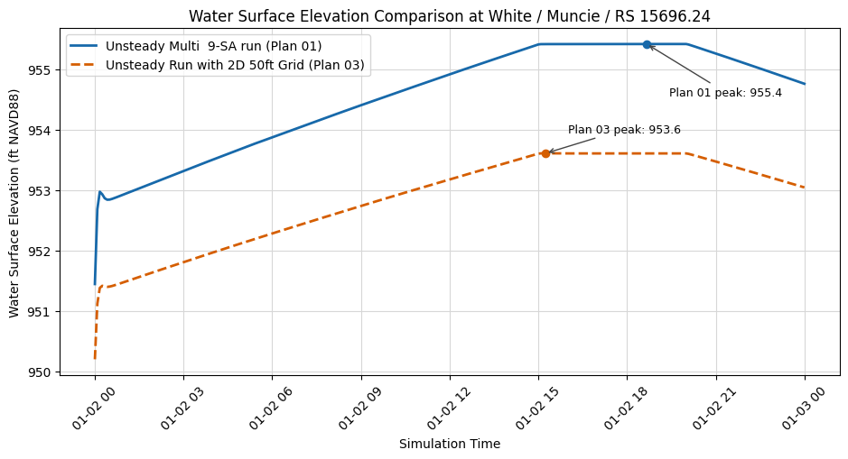
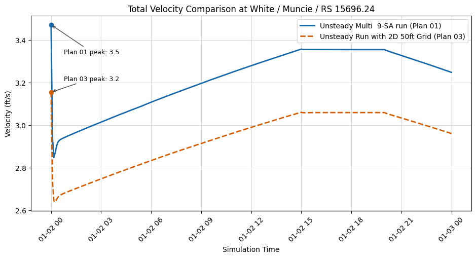
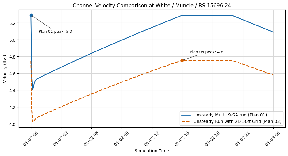
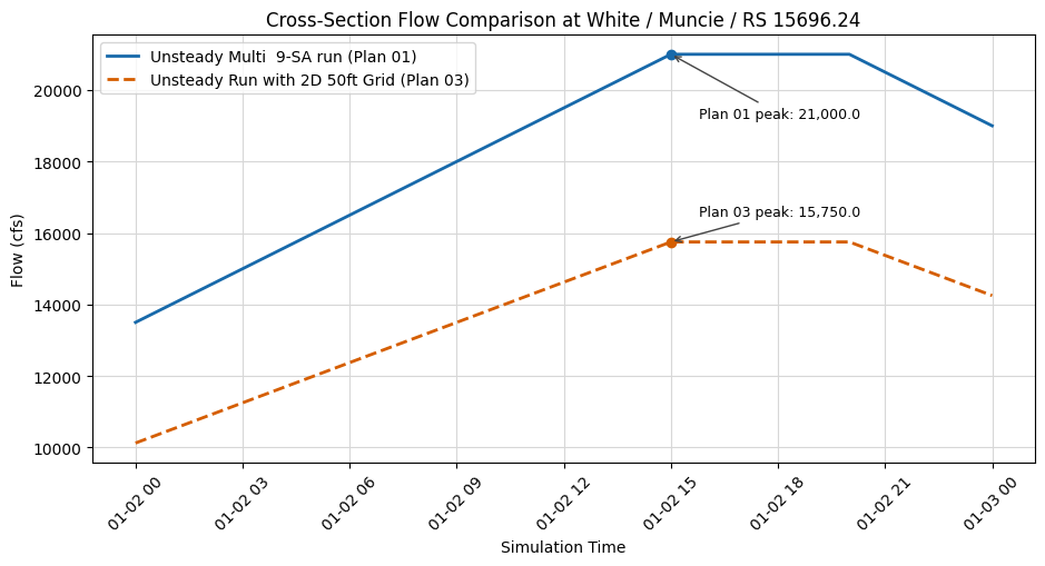
Summary of Unsteady Flow Operations

In this notebook, we've covered the following unsteady flow operations using RAS Commander:

1. Project Initialization: We initialized a HEC-RAS project to work with
2. Boundary Extraction: We extracted boundary conditions and tables from unsteady flow files
3. Boundary Analysis: We inspected and understood boundary condition structures
4. Flow Title Updates: We modified the title of an unsteady flow file
5. Restart Settings: We configured restart file settings for continuing simulations
6. Table Extraction: We extracted flow tables for analysis
7. Table Modification: We modified a flow table and wrote it back to the file
8. Application: We created a plan using our modified unsteady flow and computed results

Key Classes and Functions Used

• RasUnsteady.extract_boundary_and_tables(): Extract boundary conditions and tables
• RasUnsteady.print_boundaries_and_tables(): Display formatted boundary information
• RasUnsteady.update_flow_title(): Modify the flow title
• RasUnsteady.update_restart_settings(): Configure restart options
• RasUnsteady.extract_tables(): Extract tables from unsteady flow files
• RasUnsteady.identify_tables(): Identify table locations in file
• RasUnsteady.parse_fixed_width_table(): Parse fixed-width tables
• RasUnsteady.write_table_to_file(): Write modified tables back to file
• RasUnsteady.delete_boundary(): Remove a non-required Boundary Location= block with backup and boundaries_df refresh

Next Steps

To further explore unsteady flow operations with RAS Commander, consider:

1. Advanced Flow Modifications: Create scripts that systematically modify flow hydrographs
2. Sensitivity Analysis: Create variations of unsteady flows to assess model sensitivity
3. Batch Processing: Process multiple unsteady flow files for scenario analysis
4. Custom Boundary Conditions: Create unsteady flows from external data sources
5. Results Analysis: Compare results from different unsteady flow scenarios

These advanced topics can be explored by building on the foundation established in this notebook.