DSS Boundary Extraction
!pip install --upgrade ras-commander
Import the ras-commander package
from ras_commander import *
Overview
This notebook demonstrates extracting boundary condition data from HEC-DSS files. DSS (Data Storage System) is HEC's standard format for time-series data.
What You'll Learn
- Read DSS catalog and pathname structure
- Extract time series for specific pathnames
- Convert DSS data to pandas DataFrames
- Validate boundary condition completeness
LLM Forward Approach
- Verification: Check against DSS-Vue
- Audit Trail: Save extracted data to CSV
- Quality Checks: Validate time coverage and value ranges
Reference Documentation
Understanding DSS Pathname Structure
DSS pathnames uniquely identify time series using a 6-part format:
Part Meanings: - A: Project/Basin name - B: Location (station, reach, cross section) - C: Parameter (FLOW, STAGE, PRECIP, etc.) - D: Start date (e.g., 01JAN2020) - E: Time interval (1HOUR, 1DAY, IR-CENTURY for irregular) - F: Version or source (OBS, SIM, FORECAST)
Example: //BALD_EAGLE/MILESBURG/FLOW/01JAN2020/1HOUR/OBS/
Common Issues
Issue: Pathname not found in DSS file
- Fix: Use RasDss.get_catalog() to list available pathnames
Issue: Time series has gaps - Fix: Plot time series, identify gaps, fill or interpolate
Issue: Units mismatch - Fix: Convert units during extraction or in unsteady flow file
# =============================================================================
# DEVELOPMENT MODE TOGGLE
# =============================================================================
USE_LOCAL_SOURCE = True  # <-- TOGGLE THIS

if USE_LOCAL_SOURCE:
    import sys
    from pathlib import Path
    local_path = str(Path.cwd().parent)
    if local_path not in sys.path:
        sys.path.insert(0, local_path)
    print(f"📁 LOCAL SOURCE MODE: Loading from {local_path}/ras_commander")
else:
    print("📦 PIP PACKAGE MODE: Loading installed ras-commander")

# Import ras-commander
from ras_commander import init_ras_project, RasExamples, RasDss

# Additional imports
import pandas as pd
import numpy as np
import matplotlib.pyplot as plt

# Verify which version loaded
import ras_commander
print(f"✓ Loaded: {ras_commander.__file__}")
📁 LOCAL SOURCE MODE: Loading from c:\GH\ras-commander/ras_commander
✓ Loaded: c:\GH\ras-commander\ras_commander\__init__.py
Parameters
Configure these values to customize the notebook for your project.
# =============================================================================
# PARAMETERS - Edit these to customize the notebook
# =============================================================================
from pathlib import Path

# Project Configuration
PROJECT_NAME = "BaldEagleCrkMulti2D"  # Example project with DSS boundary conditions
RAS_VERSION = "7.0"                    # HEC-RAS version (6.3, 6.5, 6.6, etc.)

# Execution Settings
PLAN = "07"                            # Plan number with DSS boundaries
NUM_CORES = 4                          # CPU cores for 2D computation
RUN_SUFFIX = "310"                     # Suffix for run folder
DSS Boundary Condition Extraction
This notebook demonstrates how to extract DSS (Data Storage System) boundary condition data from HEC-RAS projects using ras-commander.
Example Project: BaldEagleCrkMulti2D, Plan 07
Features Demonstrated
- Reading DSS file catalogs
- Extracting individual time series
- Automatic boundary condition extraction
- Plotting DSS boundary data
# DSS operations require pyjnius which should be installed automatically
# Uncomment below if you need to install it manually:
# !pip install pyjnius
Step 1: Extract Example Project
Extract the Bald Eagle Creek Multi-2D example project which contains DSS boundary conditions.
# Extract example project with DSS boundary conditions
project_path = RasExamples.extract_project(PROJECT_NAME, suffix=RUN_SUFFIX)
print(f"Project extracted to: {project_path}")
2026-01-12 00:10:32 - ras_commander.RasExamples - INFO - Found zip file: C:\GH\ras-commander\examples\Example_Projects_6_6.zip
2026-01-12 00:10:32 - ras_commander.RasExamples - INFO - Loading project data from CSV...
2026-01-12 00:10:32 - ras_commander.RasExamples - INFO - Loaded 68 projects from CSV.
2026-01-12 00:10:32 - ras_commander.RasExamples - INFO - ----- RasExamples Extracting Project -----
2026-01-12 00:10:32 - ras_commander.RasExamples - INFO - Extracting project 'BaldEagleCrkMulti2D' as 'BaldEagleCrkMulti2D_310'
2026-01-12 00:10:34 - ras_commander.RasExamples - INFO - Successfully extracted project 'BaldEagleCrkMulti2D' to C:\GH\ras-commander\examples\example_projects\BaldEagleCrkMulti2D_310


Project extracted to: C:\GH\ras-commander\examples\example_projects\BaldEagleCrkMulti2D_310
Step 2: Initialize Project
Initialize the HEC-RAS project to access boundary condition data.
# Initialize project
ras = init_ras_project(project_path, RAS_VERSION)

print(f"\nProject: {ras.project_name}")
print(f"Plans: {len(ras.plan_df)}")
print(f"Boundaries: {len(ras.boundaries_df)}")
2026-01-12 00:10:34 - ras_commander.RasMap - INFO - Successfully parsed RASMapper file: C:\GH\ras-commander\examples\example_projects\BaldEagleCrkMulti2D_310\BaldEagleDamBrk.rasmap
2026-01-12 00:10:34 - ras_commander.RasPrj - INFO - Updated results_df with 11 plan(s)


Project: BaldEagleDamBrk
Plans: 11
Boundaries: 51
Step 3: Examine Boundary Conditions
View boundary conditions and identify which are defined by DSS files.
# Show boundaries for the plan with DSS data
plan_boundaries = ras.boundaries_df[ras.boundaries_df['unsteady_number'] == PLAN].copy()

print(f"Plan {PLAN} has {len(plan_boundaries)} boundary conditions\n")

# Show DSS-defined boundaries (handle string 'True' values)
dss_boundaries = plan_boundaries[plan_boundaries['Use DSS'] == 'True']
print(f"DSS-defined boundaries: {len(dss_boundaries)}\n")

# Display key columns if DSS boundaries exist
if len(dss_boundaries) > 0:
    display_cols = ['boundary_condition_number', 'bc_type', 'Use DSS', 'DSS File', 'DSS Path']
    print(dss_boundaries[display_cols].to_string())
else:
    print("No DSS boundaries found for this plan.")
Plan 07 has 10 boundary conditions

DSS-defined boundaries: 7

   boundary_condition_number                            bc_type Use DSS              DSS File                                                       DSS Path
0                          1                    Flow Hydrograph    True  Bald_Eagle_Creek.dss            //BALD EAGLE 40/FLOW/01JAN1999/15MIN/RUN:PMF-EVENT/
2                          3          Lateral Inflow Hydrograph    True  Bald_Eagle_Creek.dss            //FISHING CREEK/FLOW/01JAN1999/15MIN/RUN:PMF-EVENT/
4                          5  Uniform Lateral Inflow Hydrograph    True  Bald_Eagle_Creek.dss          //RESERVOIR LOCAL/FLOW/01JAN1999/15MIN/RUN:PMF-EVENT/
5                          6  Uniform Lateral Inflow Hydrograph    True  Bald_Eagle_Creek.dss  //LOCAL DOWNSTREAM OF DAM/FLOW/01JAN1999/15MIN/RUN:PMF-EVENT/
6                          7          Lateral Inflow Hydrograph    True  Bald_Eagle_Creek.dss              //MARSH CREEK/FLOW/01JAN1999/15MIN/RUN:PMF-EVENT/
7                          8          Lateral Inflow Hydrograph    True  Bald_Eagle_Creek.dss         //BEECH CREEK FLOW/FLOW/01JAN1999/15MIN/RUN:PMF-EVENT/
8                          9  Uniform Lateral Inflow Hydrograph    True  Bald_Eagle_Creek.dss         //BALD EAGLE LOCAL/FLOW/01JAN1999/15MIN/RUN:PMF-EVENT/
DSS Path Components
The new dss_part_* columns parse the DSS pathname into individual components for easy access:
| Column | DSS Part | Description |
|---|---|---|
dss_part_a |
A-part | Location/subbasin (HMS basin name) |
dss_part_b |
B-part | Parameter (FLOW, STAGE) |
dss_part_c |
C-part | Date reference |
dss_part_d |
D-part | Time interval |
dss_part_e |
E-part | Run identifier |
dss_part_f |
F-part | Additional ID (optional) |
# Display parsed DSS path components
if 'dss_part_a' in dss_boundaries.columns:
    print("Parsed DSS Path Components:")
    print("=" * 100)

    component_cols = ['bc_type', 'dss_part_a', 'dss_part_b', 'dss_part_c', 'dss_part_d', 'dss_part_e']
    available_cols = [c for c in component_cols if c in dss_boundaries.columns]
    display(dss_boundaries[available_cols])

    # Show unique HMS subbasins (A-part)
    unique_basins = dss_boundaries['dss_part_a'].dropna().unique()
    print(f"\nUnique HMS Subbasins (from A-part): {len(unique_basins)}")
    for basin in unique_basins:
        count = (dss_boundaries['dss_part_a'] == basin).sum()
        print(f"  - {basin}: {count} boundary(s)")
else:
    print("Note: dss_part_* columns not available - update ras-commander to latest version")
Step 4: Inspect DSS File
Examine what's in the DSS file before extracting data.
# Get DSS file path
dss_file = project_path / "Bald_Eagle_Creek.dss"

if dss_file.exists():
    # Get file info
    info = RasDss.get_info(dss_file)

    print(f"DSS File: {info['filename']}")
    print(f"Size: {info['file_size_mb']:.2f} MB")
    print(f"Total paths: {info['total_paths']}")

    print(f"\nFirst 10 paths:")
    catalog = RasDss.get_catalog(dss_file)
    for i, path in enumerate(catalog[:10]):
        print(f"  {i+1}. {path}")
else:
    print(f"DSS file not found: {dss_file}")
Configuring Java VM for DSS operations...
  Found Java: C:\Program Files\Java\jre1.8.0_471
[OK] Java VM configured
DSS File: Bald_Eagle_Creek.dss
Size: 29.27 MB
Total paths: 1270

First 10 paths:
  1. pathname
Step 5: Extract Single Time Series
Demonstrate extracting a single DSS time series.
| unsteady_number | boundary_condition_number | river_reach_name | river_station | storage_area_name | pump_station_name | bc_type | hydrograph_type | Interval | DSS File | ... | Flow Title | Program Version | Use Restart | Precipitation Mode | Wind Mode | Met BC=Precipitation|Mode | Met BC=Evapotranspiration|Mode | Met BC=Precipitation|Expanded View | Met BC=Precipitation|Constant Units | Met BC=Precipitation|Gridded Source | |
|---|---|---|---|---|---|---|---|---|---|---|---|---|---|---|---|---|---|---|---|---|---|
| 0 | 07 | 1 | Bald Eagle Cr. | Lock Haven | 137520 | Flow Hydrograph | Flow Hydrograph | 1HOUR | Bald_Eagle_Creek.dss | ... | PMF with Multi 2D Areas | 5.00 | 0 | NaN | NaN | NaN | NaN | NaN | NaN | NaN | |
| 2 | 07 | 3 | Bald Eagle Cr. | Lock Haven | 28519 | Lateral Inflow Hydrograph | Lateral Inflow Hydrograph | 1HOUR | Bald_Eagle_Creek.dss | ... | PMF with Multi 2D Areas | 5.00 | 0 | NaN | NaN | NaN | NaN | NaN | NaN | NaN | |
| 4 | 07 | 5 | Bald Eagle Cr. | Lock Haven | 136948 | 82303 | Uniform Lateral Inflow Hydrograph | Uniform Lateral Inflow Hydrograph | 1HOUR | Bald_Eagle_Creek.dss | ... | PMF with Multi 2D Areas | 5.00 | 0 | NaN | NaN | NaN | NaN | NaN | NaN | NaN |
| 5 | 07 | 6 | Bald Eagle Cr. | Lock Haven | 80720 | 67130 | Uniform Lateral Inflow Hydrograph | Uniform Lateral Inflow Hydrograph | 1HOUR | Bald_Eagle_Creek.dss | ... | PMF with Multi 2D Areas | 5.00 | 0 | NaN | NaN | NaN | NaN | NaN | NaN | NaN |
| 6 | 07 | 7 | Bald Eagle Cr. | Lock Haven | 76865 | Lateral Inflow Hydrograph | Lateral Inflow Hydrograph | 1HOUR | Bald_Eagle_Creek.dss | ... | PMF with Multi 2D Areas | 5.00 | 0 | NaN | NaN | NaN | NaN | NaN | NaN | NaN | |
| 7 | 07 | 8 | Bald Eagle Cr. | Lock Haven | 67130 | Lateral Inflow Hydrograph | Lateral Inflow Hydrograph | 1HOUR | Bald_Eagle_Creek.dss | ... | PMF with Multi 2D Areas | 5.00 | 0 | NaN | NaN | NaN | NaN | NaN | NaN | NaN | |
| 8 | 07 | 9 | Bald Eagle Cr. | Lock Haven | 66041 | 1 | Uniform Lateral Inflow Hydrograph | Uniform Lateral Inflow Hydrograph | 1HOUR | Bald_Eagle_Creek.dss | ... | PMF with Multi 2D Areas | 5.00 | 0 | NaN | NaN | NaN | NaN | NaN | NaN | NaN |
7 rows × 29 columns
if len(dss_boundaries) > 0:
    # Get first DSS boundary
    first_dss = dss_boundaries.iloc[0]

    print(f"Boundary Type: {first_dss['bc_type']}")
    print(f"DSS Path: {first_dss['DSS Path']}")

    # Extract time series
    dss_file_path = project_path / first_dss['DSS File']
    df_ts = RasDss.read_timeseries(dss_file_path, first_dss['DSS Path'])

    print(f"\nExtracted {len(df_ts)} data points")
    print(f"Date range: {df_ts.index.min()} to {df_ts.index.max()}")
    print(f"Value range: {df_ts['value'].min():.2f} to {df_ts['value'].max():.2f}")
    print(f"Units: {df_ts.attrs.get('units', 'N/A')}")

    # Display first/last rows
    print(f"\nFirst 5 rows:")
    display(df_ts.head())

    print(f"\nLast 5 rows:")
    display(df_ts.tail())
else:
    print("No DSS boundaries to extract - run previous cells first.")
Boundary Type: Flow Hydrograph
DSS Path: //BALD EAGLE 40/FLOW/01JAN1999/15MIN/RUN:PMF-EVENT/

Extracted 673 data points
Date range: 1999-01-01 00:00:00 to 1999-01-08 00:00:00
Value range: 719.78 to 193738.20
Units: CFS

First 5 rows:
| value | |
|---|---|
| datetime | |
| 1999-01-01 00:00:00 | 804.059996 |
| 1999-01-01 00:15:00 | 804.055225 |
| 1999-01-01 00:30:00 | 803.989415 |
| 1999-01-01 00:45:00 | 803.618691 |
| 1999-01-01 01:00:00 | 802.505521 |
Last 5 rows:
| value | |
|---|---|
| datetime | |
| 1999-01-07 23:00:00 | 3747.890234 |
| 1999-01-07 23:15:00 | 3733.991294 |
| 1999-01-07 23:30:00 | 3720.143897 |
| 1999-01-07 23:45:00 | 3706.347853 |
| 1999-01-08 00:00:00 | 3692.602971 |
Step 6: Plot Time Series
Visualize the extracted DSS boundary condition data.
# Extract all DSS boundary time series for the plan
enhanced_boundaries = RasDss.extract_boundary_timeseries(
    plan_boundaries,
    ras_object=ras
)

# Show results
print(f"\nExtraction complete!")
print(f"Total boundaries: {len(enhanced_boundaries)}")

# Count DSS-defined boundaries (handle string 'True')
dss_count = (enhanced_boundaries['Use DSS'] == 'True').sum()
print(f"DSS-defined: {dss_count}")

# Show extracted data summary
print(f"\nDSS Boundary Summary:")
print("-" * 80)
for idx, row in enhanced_boundaries.iterrows():
    # Check if DSS boundary (handle string 'True')
    is_dss = row['Use DSS'] == 'True'
    if is_dss and row['dss_timeseries'] is not None:
        df = row['dss_timeseries']
        print(f"\n{row['bc_type']}:")
        print(f"  Location: {row['river_reach_name']} RS {row['river_station']}")
        print(f"  DSS Path: {row['DSS Path']}")
        print(f"  Points: {len(df)}")
        print(f"  Date range: {df.index.min()} to {df.index.max()}")
        print(f"  Value range: {df['value'].min():.2f} to {df['value'].max():.2f} {df.attrs.get('units', '')}")
2026-01-12 00:10:34 - ras_commander.dss.RasDss - INFO - Found 7 DSS-defined boundaries
2026-01-12 00:10:34 - ras_commander.dss.RasDss - INFO - Row 0: Extracted 673 points from Bald_Eagle_Creek.dss
2026-01-12 00:10:34 - ras_commander.dss.RasDss - INFO - Row 2: Extracted 673 points from Bald_Eagle_Creek.dss
2026-01-12 00:10:34 - ras_commander.dss.RasDss - INFO - Row 4: Extracted 673 points from Bald_Eagle_Creek.dss
2026-01-12 00:10:34 - ras_commander.dss.RasDss - INFO - Row 5: Extracted 673 points from Bald_Eagle_Creek.dss
2026-01-12 00:10:34 - ras_commander.dss.RasDss - INFO - Row 6: Extracted 673 points from Bald_Eagle_Creek.dss
2026-01-12 00:10:34 - ras_commander.dss.RasDss - INFO - Row 7: Extracted 673 points from Bald_Eagle_Creek.dss
2026-01-12 00:10:34 - ras_commander.dss.RasDss - INFO - Row 8: Extracted 673 points from Bald_Eagle_Creek.dss
2026-01-12 00:10:34 - ras_commander.dss.RasDss - INFO - Extraction complete: 7 success, 0 failed
Extraction complete!
Total boundaries: 10
DSS-defined: 7
DSS Boundary Summary:
--------------------------------------------------------------------------------
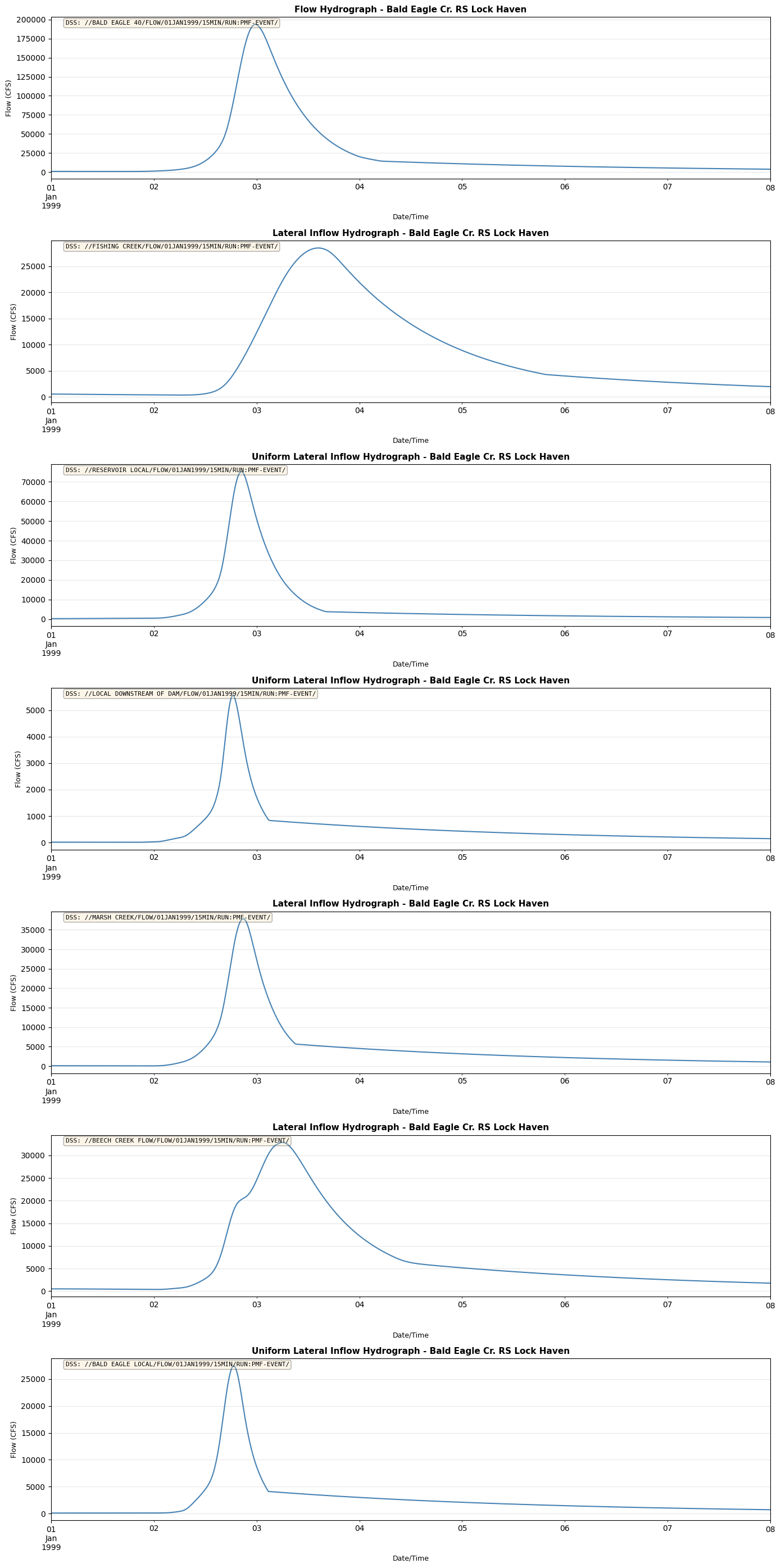
Flow Hydrograph:
Location: Bald Eagle Cr. RS Lock Haven
DSS Path: //BALD EAGLE 40/FLOW/01JAN1999/15MIN/RUN:PMF-EVENT/
Points: 673
Date range: 1999-01-01 00:00:00 to 1999-01-08 00:00:00
Value range: 719.78 to 193738.20 CFS
Lateral Inflow Hydrograph:
Location: Bald Eagle Cr. RS Lock Haven
DSS Path: //FISHING CREEK/FLOW/01JAN1999/15MIN/RUN:PMF-EVENT/
Points: 673
Date range: 1999-01-01 00:00:00 to 1999-01-08 00:00:00
Value range: 345.89 to 28510.08 CFS
Uniform Lateral Inflow Hydrograph:
Location: Bald Eagle Cr. RS Lock Haven
DSS Path: //RESERVOIR LOCAL/FLOW/01JAN1999/15MIN/RUN:PMF-EVENT/
Points: 673
Date range: 1999-01-01 00:00:00 to 1999-01-08 00:00:00
Value range: 209.15 to 75262.30 CFS
Uniform Lateral Inflow Hydrograph:
Location: Bald Eagle Cr. RS Lock Haven
DSS Path: //LOCAL DOWNSTREAM OF DAM/FLOW/01JAN1999/15MIN/RUN:PMF-EVENT/
Points: 673
Date range: 1999-01-01 00:00:00 to 1999-01-08 00:00:00
Value range: 9.98 to 5568.15 CFS
Lateral Inflow Hydrograph:
Location: Bald Eagle Cr. RS Lock Haven
DSS Path: //MARSH CREEK/FLOW/01JAN1999/15MIN/RUN:PMF-EVENT/
Points: 673
Date range: 1999-01-01 00:00:00 to 1999-01-08 00:00:00
Value range: 94.61 to 37820.33 CFS
Lateral Inflow Hydrograph:
Location: Bald Eagle Cr. RS Lock Haven
DSS Path: //BEECH CREEK FLOW/FLOW/01JAN1999/15MIN/RUN:PMF-EVENT/
Points: 673
Date range: 1999-01-01 00:00:00 to 1999-01-08 00:00:00
Value range: 382.69 to 32872.19 CFS
Uniform Lateral Inflow Hydrograph:
Location: Bald Eagle Cr. RS Lock Haven
DSS Path: //BALD EAGLE LOCAL/FLOW/01JAN1999/15MIN/RUN:PMF-EVENT/
Points: 673
Date range: 1999-01-01 00:00:00 to 1999-01-08 00:00:00
Value range: 100.19 to 27428.17 CFS
Step 7: Extract ALL Boundary DSS Data
Use the extract_boundary_timeseries() function to automatically extract ALL DSS boundary data in one call.
# Count boundary types
print("Boundary Definition Summary:")
print("=" * 80)

# Handle string 'True'/'False' values
manual_bc = enhanced_boundaries[
    (enhanced_boundaries['Use DSS'] != 'True') | (enhanced_boundaries['Use DSS'].isna())
]
dss_bc = enhanced_boundaries[enhanced_boundaries['Use DSS'] == 'True']

print(f"\nManual boundaries (defined in .u## file): {len(manual_bc)}")
if len(manual_bc) > 0:
    print("  Types:")
    for bc_type, count in manual_bc['bc_type'].value_counts().items():
        print(f"    - {bc_type}: {count}")

print(f"\nDSS boundaries (defined in DSS file): {len(dss_bc)}")
if len(dss_bc) > 0:
    print("  Types:")
    for bc_type, count in dss_bc['bc_type'].value_counts().items():
        print(f"    - {bc_type}: {count}")

print(f"\nTotal boundaries: {len(enhanced_boundaries)}")
Boundary Definition Summary:
================================================================================

Manual boundaries (defined in .u## file): 3
  Types:
    - Gate Opening: 1
    - Lateral Inflow Hydrograph: 1
    - Normal Depth: 1

DSS boundaries (defined in DSS file): 7
  Types:
    - Lateral Inflow Hydrograph: 3
    - Uniform Lateral Inflow Hydrograph: 3
    - Flow Hydrograph: 1

Total boundaries: 10
Step 8: Compare Manual vs DSS Boundaries
Show the difference between manually-defined and DSS-defined boundary conditions.
# Get all successfully extracted DSS boundaries
successful_dss = enhanced_boundaries[
    ((enhanced_boundaries['Use DSS'] == True) | (enhanced_boundaries['Use DSS'] == 'True')) &
    (enhanced_boundaries['dss_timeseries'].notna())
]

if len(successful_dss) > 0:
    # Create subplots
    n_plots = len(successful_dss)
    fig, axes = plt.subplots(n_plots, 1, figsize=(14, 4*n_plots))

    if n_plots == 1:
        axes = [axes]

    for ax, (idx, row) in zip(axes, successful_dss.iterrows()):
        df = row['dss_timeseries']

        # Plot
        df['value'].plot(ax=ax, linewidth=1.5, color='steelblue')

        # Format
        title = f"{row['bc_type']} - {row['river_reach_name']} RS {row['river_station']}"
        ax.set_title(title, fontsize=11, fontweight='bold')
        ax.set_xlabel('Date/Time', fontsize=9)
        ax.set_ylabel(f"Flow ({df.attrs.get('units', '')})", fontsize=9)
        ax.grid(True, alpha=0.3)

        # Add DSS path as text
        ax.text(0.02, 0.98, f"DSS: {row['DSS Path']}",
                transform=ax.transAxes, fontsize=8,
                verticalalignment='top', family='monospace',
                bbox=dict(boxstyle='round', facecolor='wheat', alpha=0.3))

    plt.tight_layout()
    plt.show()
else:
    print("No successful DSS extractions to plot")
Step 9: Plot Multiple DSS Boundaries
Create a multi-panel plot showing all DSS boundary conditions.
# Export to CSV (without the DataFrame column)
export_df = enhanced_boundaries.drop(columns=['dss_timeseries']).copy()

# Add summary statistics for DSS boundaries
for idx, row in enhanced_boundaries.iterrows():
    is_dss = row['Use DSS'] == 'True'
    if is_dss and row['dss_timeseries'] is not None:
        df = row['dss_timeseries']
        export_df.at[idx, 'dss_points'] = len(df)
        export_df.at[idx, 'dss_mean'] = df['value'].mean()
        export_df.at[idx, 'dss_max'] = df['value'].max()
        export_df.at[idx, 'dss_min'] = df['value'].min()

# Save
output_file = project_path / "boundaries_with_dss_summary.csv"
export_df.to_csv(output_file, index=False)
print(f"Exported to: {output_file}")

# Show summary
dss_summary_cols = ['bc_type', 'Use DSS', 'dss_points', 'dss_mean', 'dss_max', 'dss_min']
available_cols = [c for c in dss_summary_cols if c in export_df.columns]
print(f"\nDSS Boundary Statistics:")

# Filter for DSS boundaries
dss_summary = export_df[export_df['Use DSS'] == 'True'][available_cols]
display(dss_summary)
Exported to: C:\GH\ras-commander\examples\example_projects\BaldEagleCrkMulti2D_310\boundaries_with_dss_summary.csv

DSS Boundary Statistics:
| bc_type | Use DSS | dss_points | dss_mean | dss_max | dss_min | |
|---|---|---|---|---|---|---|
| 0 | Flow Hydrograph | True | 673.0 | 23749.776843 | 193738.197396 | 719.775321 |
| 2 | Lateral Inflow Hydrograph | True | 673.0 | 7554.055251 | 28510.083069 | 345.889757 |
| 4 | Uniform Lateral Inflow Hydrograph | True | 673.0 | 6448.671063 | 75262.300507 | 209.150354 |
| 5 | Uniform Lateral Inflow Hydrograph | True | 673.0 | 539.962137 | 5568.152787 | 9.979876 |
| 6 | Lateral Inflow Hydrograph | True | 673.0 | 4343.093777 | 37820.325998 | 94.606990 |
| 7 | Lateral Inflow Hydrograph | True | 673.0 | 6971.806773 | 32872.193876 | 382.693009 |
| 8 | Uniform Lateral Inflow Hydrograph | True | 673.0 | 2710.452795 | 27428.172923 | 100.189004 |
Step 10: Export Boundary Data
Save extracted boundary condition data for further analysis.
# Export individual DSS time series to CSV files
if len(dss_bc) > 0:
    for idx, row in enhanced_boundaries.iterrows():
        is_dss = row['Use DSS'] == 'True'
        if is_dss and row['dss_timeseries'] is not None:
            df = row['dss_timeseries']
            bc_name = f"{row['bc_type']}_{row['boundary_condition_number']}".replace(' ', '_')
            ts_file = project_path / f"{bc_name}_timeseries.csv"
            df.to_csv(ts_file)
            print(f"Exported: {ts_file.name}")
else:
    print("No DSS boundaries to export.")
Exported: Flow_Hydrograph_1_timeseries.csv
Exported: Lateral_Inflow_Hydrograph_3_timeseries.csv
Exported: Uniform_Lateral_Inflow_Hydrograph_5_timeseries.csv
Exported: Uniform_Lateral_Inflow_Hydrograph_6_timeseries.csv
Exported: Lateral_Inflow_Hydrograph_7_timeseries.csv
Exported: Lateral_Inflow_Hydrograph_8_timeseries.csv
Exported: Uniform_Lateral_Inflow_Hydrograph_9_timeseries.csv
Step 11: Access Individual DSS Time Series
Access extracted data from the enhanced boundaries_df.
# Access specific boundary by index
if len(successful_dss) > 0:
    # Get first successful DSS boundary
    idx = successful_dss.index[0]
    boundary_data = enhanced_boundaries.loc[idx, 'dss_timeseries']

    print(f"Accessing DSS data for boundary {idx}:")
    print(f"  Type: {enhanced_boundaries.loc[idx, 'bc_type']}")
    print(f"  Data points: {len(boundary_data)}")

    # Show statistics
    print(f"\nData statistics:")
    print(boundary_data['value'].describe())

    # Access metadata
    print(f"\nMetadata:")
    for key, value in boundary_data.attrs.items():
        print(f"  {key}: {value}")
Accessing DSS data for boundary 0:
  Type: Flow Hydrograph
  Data points: 673

Data statistics:
count       673.000000
mean      23749.776843
std       42452.303066
min         719.775321
25%        4332.272683
50%        7792.191249
75%       14070.993090
max      193738.197396
Name: value, dtype: float64

Metadata:
  pathname: //BALD EAGLE 40/FLOW/01JAN1999/15MIN/RUN:PMF-EVENT/
  units: CFS
  type: INST-VAL
  interval: 15
  dss_file: C:\GH\ras-commander\examples\example_projects\BaldEagleCrkMulti2D_310\Bald_Eagle_Creek.dss
Summary
This notebook demonstrated:
1. ✅ Reading DSS file catalogs
2. ✅ Extracting individual time series from DSS files
3. ✅ Automatic extraction of ALL DSS boundary data with extract_boundary_timeseries()
4. ✅ Plotting and analyzing DSS data
5. ✅ Exporting results
Key Features
- Unified API - Same DataFrame structure for manual and DSS boundaries
- Automatic extraction - One function call extracts all DSS data
- V6 and V7 support - Works with both DSS formats
- Auto-download - HEC Monolith libraries downloaded automatically on first use
Next Steps
- Use extracted data for boundary condition analysis
- Compare DSS vs manual boundary definitions
- Modify DSS data and write back to files (future enhancement)
- Integrate DSS data with HEC-RAS model workflows