1D Channel Capacity Analysis
This notebook demonstrates the HdfChannelCapacity class for analyzing 1D channel capacity
using WSE results and bank station elevations. Channel capacity is determined by comparing
water surface elevations from multiple AEP storm profiles against bank elevations at each
cross section, then aggregating the result into 0.25-mile channel segments.
Capacity Levels:
| Level | Category | Description |
|---|---|---|
| 1 | <=2-yr | Contains 50% AEP (2-year) or less |
| 2 | 5-yr | Contains 20% AEP (5-year) |
| 3 | 10-yr | Contains 10% AEP (10-year) |
| 4 | 25-yr | Contains 4% AEP (25-year) |
| 5 | 50-yr | Contains 2% AEP (50-year) |
| 6 | 100-yr | Contains 1% AEP (100-year) |
| 7 | >=500-yr | Contains 0.2% AEP (500-year) |
What you'll learn: - Extract bank elevations from geometry HDF - Extract individual steady-state profile WSE from a single plan HDF - Determine channel capacity level at each cross section - Aggregate capacity into channel segments - Generate system-wide capacity summaries - Compare existing vs proposed conditions
Data Source: FEMA BLE model (Lower Colorado-Cummins, HUC 12090301), SHILOH BRANCH reach with 40 cross sections and 7 steady-state flow profiles.
# =============================================================================
# DEVELOPMENT MODE TOGGLE
# =============================================================================
USE_LOCAL_SOURCE = True  # <-- TOGGLE THIS
import os
import logging
os.environ.setdefault("NUMEXPR_MAX_THREADS", "8")
logging.disable(logging.CRITICAL)
logging.getLogger().setLevel(logging.ERROR)
logging.getLogger("numexpr").setLevel(logging.ERROR)

if USE_LOCAL_SOURCE:
    import sys
    from pathlib import Path
    repo_candidates = [Path.cwd(), Path.cwd().parent]
    local_path = str(next((p for p in repo_candidates if (p / "ras_commander").exists()), Path.cwd()))
    if local_path not in sys.path:
        sys.path.insert(0, local_path)
    print("LOCAL SOURCE MODE: Loading ras-commander from the active workspace")
else:
    print("PIP PACKAGE MODE: Loading installed ras-commander")

from ras_commander import init_ras_project, RasCmdr, RasPlan
from ras_commander.hdf.HdfChannelCapacity import (
    HdfChannelCapacity, STORM_ORDER, LEVEL_TO_CATEGORY
)
from ras_commander.sources.federal import RasEbfeModels
logging.getLogger().setLevel(logging.ERROR)
logging.getLogger("ras_commander").setLevel(logging.ERROR)
import ras_commander
print(f"ras-commander version: {getattr(ras_commander, '__version__', 'local source')}")

import numpy as np
import pandas as pd
import matplotlib.pyplot as plt
from pathlib import Path
LOCAL SOURCE MODE: Loading ras-commander from the active workspace


ras-commander version: 0.96.0
Setup: BLE Model Preparation
We use a FEMA Base Level Engineering (BLE) reach model — SHILOH BRANCH from the Lower Colorado-Cummins study (HUC 12090301). BLE models are steady-state with 7 flow profiles representing different AEP events.
RasEbfeModels.organize_model("lower-colorado-cummins") handles downloading the 290.7 MB BLE archive from S3 and organizing the selected reach into the shared delivery workspace. Since BLE models were built with HEC-RAS 4.x, we re-run with HEC-RAS 6.5 to generate HDF output files needed for analysis.
Saved-run interpretation: 1D BLE reach projects may not include .rasmap files, project CRS metadata, terrain, or land-cover layers. Those warnings are expected for this 1D steady workflow and do not invalidate the HDF-based channel-capacity analysis. HDF logs may also include non-blocking metadata warnings such as unknown simulation timestamps.
# =============================================================================
# Parameters
# =============================================================================

# Reach to extract from BLE archive (Lower Colorado-Cummins, HUC 12090301)
BLE_RIVER = "Rabbs Creek-Colorado River"
BLE_REACH_NAME = "SHILOH BRANCH"

# HEC-RAS version for re-running. Version 7.0 migrates this steady 1D BLE model
# and writes the geometry/results HDF files used by the analysis below.
RAS_VERSION = "7.0"
# BLE profile name to standard AEP mapping
# Only 5 of the 7 profiles are standard AEP events;
# '1pct_min' and '1pct_plu' are confidence bounds, excluded
BLE_TO_AEP = {
    '10-year':  '10P',   # 10% AEP
    '25-year':  '4P',    #  4% AEP
    '50-year':  '2P',    #  2% AEP
    '100-year': '1P',    #  1% AEP
    '500-year': '0.2P',  #  0.2% AEP
}

# Storm order for capacity analysis (smallest to largest)
STORM_ORDER_BLE = ['10P', '4P', '2P', '1P', '0.2P']

# Segment length for aggregation (0.25 miles = 1320 ft)
SEGMENT_LENGTH = 1320.0

print(f"Reach: {BLE_RIVER} / {BLE_REACH_NAME}")
print(f"Storm order: {STORM_ORDER_BLE}")
# Shared eBFE workspace. Override RAS_COMMANDER_EBFE_ROOT to use a different local cache.
EBFE_WORKSPACE = Path(os.environ.get("RAS_COMMANDER_EBFE_ROOT", r"H:\Testing\eBFE Model Organization"))
DOWNLOAD_ROOT = EBFE_WORKSPACE / "Downloads"
ORGANIZED_ROOT = EBFE_WORKSPACE / "Organized"
VALIDATION_ROOT = EBFE_WORKSPACE / "Validation" / "ebfe_delivery"
repo_candidates = [Path.cwd(), Path.cwd().parent]
VALIDATION_MATRIX = next(
    (candidate / "VALIDATION_MATRIX.md" for candidate in repo_candidates if (candidate / "VALIDATION_MATRIX.md").exists()),
    Path.cwd() / "VALIDATION_MATRIX.md",
)

print(f"eBFE workspace configured: {EBFE_WORKSPACE.exists()}")
print(f"Validation matrix: {VALIDATION_MATRIX.name if VALIDATION_MATRIX else 'not found'}")
# Download/cache, extract, and organize the BLE model using the shared eBFE delivery workspace.
# Auto-downloads 290.7 MB from S3 if not already cached under DOWNLOAD_ROOT.
from contextlib import redirect_stdout
import io

with redirect_stdout(io.StringIO()):
    organized = RasEbfeModels.organize_model(
        "lower-colorado-cummins",
        download_root=DOWNLOAD_ROOT,
        output_root=ORGANIZED_ROOT,
        river=BLE_RIVER,
        reach=BLE_REACH_NAME,
    )

# Project folder is under RAS Model/{River}/{Reach}/
project_folder = organized / "RAS Model" / BLE_RIVER / BLE_REACH_NAME

print(f"Organized study: {organized.name}")
print(f"Project folder: {project_folder.name}")
print(f"Validation root configured: {VALIDATION_ROOT.exists()}")
print(f"\nProject files:")
for f in sorted(project_folder.iterdir()):
    if f.is_file():
        print(f"  {f.name} ({f.stat().st_size:,} bytes)")
Organized study: LowerColoradoCummins_12090301
Project folder: SHILOH BRANCH
Validation root configured: True

Project files:
  SHILOH BRANCH.f01 (1,778 bytes)
  SHILOH BRANCH.g01 (358,968 bytes)
  SHILOH BRANCH.O01 (224,000 bytes)
  SHILOH BRANCH.p01 (3,197 bytes)
  SHILOH BRANCH.p01.comp_msgs.txt (122 bytes)
  SHILOH BRANCH.p01.hdf (735,637 bytes)
  SHILOH BRANCH.prj (591 bytes)
  SHILOH BRANCH.r01 (255,091 bytes)
  SHILOH BRANCH.xml (1,543,746 bytes)
# Initialize project
ras = init_ras_project(project_folder, RAS_VERSION)

print(f"Project: {ras.project_name}")
print(f"Plans: {len(ras.plan_df)}")
print(f"Geometry: {ras.geom_df['geom_title'].iloc[0]}")
print(f"Flow profiles: {ras.flow_df['Flow Title'].iloc[0]}")

plan_file = project_folder / f"{ras.project_name}.p01"
plan_hdf = project_folder / f"{ras.project_name}.p01.hdf"
geom_hdf = project_folder / f"{ras.project_name}.g01.hdf"

# BLE models were built with HEC-RAS 4.x. Reuse cached HDF output when present;
# otherwise enable HDF-producing run flags and compute through RasCmdr.
if plan_hdf.exists():
    print(f"\nUsing cached plan HDF: {plan_hdf.name} ({plan_hdf.stat().st_size:,} bytes)")
elif geom_hdf.exists():
    print(f"\nUsing cached geometry HDF: {geom_hdf.name} ({geom_hdf.stat().st_size:,} bytes)")
else:
    # Enable HDF output: BLE 4.x models ship with the geometry preprocessor
    # and post-processor OFF, so they produce no HDF. Use the library API
    # instead of brittle string-replace; leave the stored Program Version
    # as-is (HEC-RAS auto-migrates the 4.x model on compute). CLB-887.
    RasPlan.update_run_flags("01", geometry_preprocessor=True, post_processor=True, ras_object=ras)
    print("\nEnabled geometry preprocessor + post-processor for HDF output")

    print("Running HEC-RAS...")
    RasCmdr.compute_plan("01", ras_object=ras, force_geompre=True)

# Re-initialize to pick up HDF paths
ras = init_ras_project(project_folder, RAS_VERSION)
if not plan_hdf.exists() and geom_hdf.exists():
    plan_hdf = geom_hdf
if not plan_hdf.exists():
    raise FileNotFoundError(f"No HDF output found for {ras.project_name}. Expected {plan_hdf.name} or {geom_hdf.name}.")

# Verify HDF files created
hdf_files = list(project_folder.glob("*.hdf"))
print(f"\nHDF files generated:")
for h in hdf_files:
    print(f"  {h.name} ({h.stat().st_size:,} bytes)")
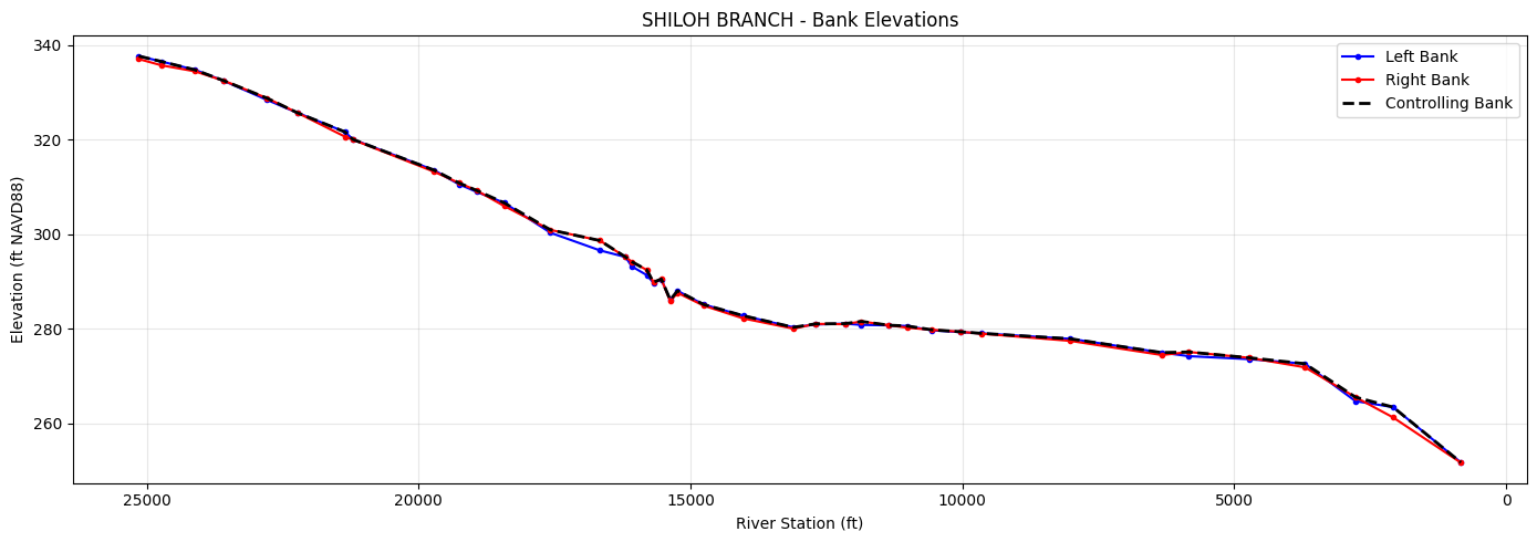
Step 1: Extract Bank Elevations
extract_bank_elevations() reads cross section geometry from the geometry HDF
and interpolates elevations at the left and right bank stations. The "controlling"
bank elevation (the higher of the two) determines where overtopping occurs.
# Get geometry HDF path
geom_hdf = project_folder / f"{ras.project_name}.g01.hdf"
if not geom_hdf.exists():
    geom_hdf = plan_hdf

bank_df = HdfChannelCapacity.extract_bank_elevations(str(geom_hdf))

print(f"Cross sections: {len(bank_df)}")
print(f"\nBank elevation range:")
print(f"  Left:  {bank_df['left_bank_elev'].min():.1f} - {bank_df['left_bank_elev'].max():.1f} ft")
print(f"  Right: {bank_df['right_bank_elev'].min():.1f} - {bank_df['right_bank_elev'].max():.1f} ft")
print(f"  Controlling: {bank_df['controlling_bank_elev'].min():.1f} - {bank_df['controlling_bank_elev'].max():.1f} ft")

bank_df.head(10)
Cross sections: 40

Bank elevation range:
  Left:  251.7 - 337.6 ft
  Right: 251.6 - 337.0 ft
  Controlling: 251.7 - 337.6 ft
| River | Reach | RS | Left Bank | Right Bank | left_bank_elev | right_bank_elev | controlling_bank_elev | thalweg_elev | channel_depth | Len Channel | |
|---|---|---|---|---|---|---|---|---|---|---|---|
| 0 | SHILOH BRANCH | Reach-1 | 25147 | 4952.600098 | 5352.399902 | 337.649994 | 337.019989 | 337.649994 | 330.920013 | 6.729980 | 418.0 |
| 1 | SHILOH BRANCH | Reach-1 | 24729 | 4725.000000 | 5036.299805 | 336.500000 | 335.700012 | 336.500000 | 329.130005 | 7.369995 | 614.0 |
| 2 | SHILOH BRANCH | Reach-1 | 24115 | 4802.799805 | 5104.299805 | 334.750000 | 334.429993 | 334.750000 | 325.149994 | 9.600006 | 534.0 |
| 3 | SHILOH BRANCH | Reach-1 | 23581 | 4924.399902 | 5204.500000 | 332.399994 | 332.440002 | 332.440002 | 323.970001 | 8.470001 | 795.0 |
| 4 | SHILOH BRANCH | Reach-1 | 22786 | 4835.700195 | 5135.700195 | 328.369995 | 328.739990 | 328.739990 | 318.380005 | 10.359985 | 553.0 |
| 5 | SHILOH BRANCH | Reach-1 | 22233 | 4796.100098 | 5056.100098 | 325.679993 | 325.679993 | 325.679993 | 316.290009 | 9.389984 | 877.0 |
| 6 | SHILOH BRANCH | Reach-1 | 21356 | 4946.299805 | 5176.399902 | 321.619995 | 320.619995 | 321.619995 | 314.910004 | 6.709991 | 148.0 |
| 7 | SHILOH BRANCH | Reach-1 | 21208 | 4944.799805 | 5225.100098 | 320.029999 | 319.970001 | 320.029999 | 314.980011 | 5.049988 | 1494.0 |
| 8 | SHILOH BRANCH | Reach-1 | 19714 | 4835.000000 | 5080.500000 | 313.519989 | 313.190002 | 313.519989 | 304.750000 | 8.769989 | 456.0 |
| 9 | SHILOH BRANCH | Reach-1 | 19258 | 4938.700195 | 5108.600098 | 310.529999 | 310.820007 | 310.820007 | 303.980011 | 6.839996 | 320.0 |
# Plot bank elevations along the channel
fig, ax = plt.subplots(figsize=(14, 5))

rs_float = bank_df['RS'].astype(float)

ax.plot(rs_float, bank_df['left_bank_elev'], 'b-o', markersize=3, label='Left Bank')
ax.plot(rs_float, bank_df['right_bank_elev'], 'r-o', markersize=3, label='Right Bank')
ax.plot(rs_float, bank_df['controlling_bank_elev'], 'k--', linewidth=2, label='Controlling Bank')

ax.set_xlabel('River Station (ft)')
ax.set_ylabel('Elevation (ft NAVD88)')
ax.set_title(f'{BLE_REACH_NAME} - Bank Elevations')
ax.legend()
ax.invert_xaxis()  # Downstream to right
ax.grid(True, alpha=0.3)
plt.tight_layout()
plt.show()
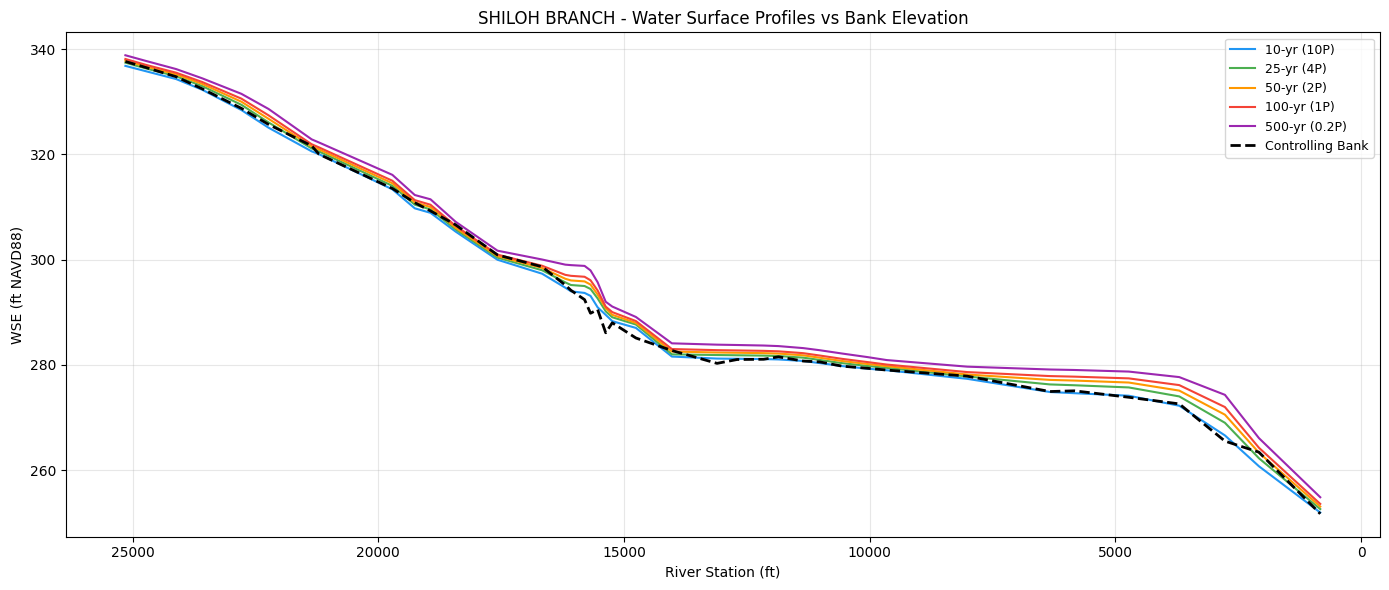
Step 2: Extract Steady-State Profile WSE
extract_steady_profile_wse() reads individual steady-state profiles from a single
plan HDF. Unlike extract_max_wse() (which collapses profiles to max), this method
preserves each profile as a separate column — essential for capacity analysis.
The BLE model has 7 profiles. We map 5 standard AEP events
# Extract all steady-state profiles from the plan HDF
plan_hdf = project_folder / f"{ras.project_name}.p01.hdf"

all_profiles = HdfChannelCapacity.extract_steady_profile_wse(str(plan_hdf))

print(f"Profiles found: {[c for c in all_profiles.columns if c not in ('River','Reach','RS')]}")
print(f"Cross sections: {len(all_profiles)}")

# Rename BLE profile names to AEP labels and select standard events
wse_df = all_profiles.rename(columns=BLE_TO_AEP)
keep_cols = ['River', 'Reach', 'RS'] + STORM_ORDER_BLE
wse_df = wse_df[keep_cols]

print(f"\nSelected AEP profiles: {STORM_ORDER_BLE}")
print(f"Excluded: 1pct_min, 1pct_plu (confidence bounds)")

wse_df.head(10)
Profiles found: ['10-year', '25-year', '50-year', '1pct_min', '100-year', '1pct_plu', '500-year']


Cross sections: 40

Selected AEP profiles: ['10P', '4P', '2P', '1P', '0.2P']
Excluded: 1pct_min, 1pct_plu (confidence bounds)
| River | Reach | RS | 10P | 4P | 2P | 1P | 0.2P | |
|---|---|---|---|---|---|---|---|---|
| 0 | SHILOH BRANCH | Reach-1 | 25147 | 336.810333 | 337.419373 | 337.794678 | 338.118896 | 338.828705 |
| 1 | SHILOH BRANCH | Reach-1 | 24729 | 335.793335 | 336.329254 | 336.679382 | 337.006317 | 337.750946 |
| 2 | SHILOH BRANCH | Reach-1 | 24115 | 334.307800 | 334.842651 | 335.201111 | 335.512787 | 336.206757 |
| 3 | SHILOH BRANCH | Reach-1 | 23581 | 332.265320 | 332.958618 | 333.370911 | 333.735413 | 334.437775 |
| 4 | SHILOH BRANCH | Reach-1 | 22786 | 328.416779 | 329.410492 | 330.002197 | 330.583191 | 331.499481 |
| 5 | SHILOH BRANCH | Reach-1 | 22233 | 325.059509 | 326.057037 | 326.748352 | 327.410858 | 328.621094 |
| 6 | SHILOH BRANCH | Reach-1 | 21356 | 320.570374 | 321.126007 | 321.525146 | 321.919586 | 322.848328 |
| 7 | SHILOH BRANCH | Reach-1 | 21208 | 320.034058 | 320.552795 | 320.937317 | 321.326630 | 322.259430 |
| 8 | SHILOH BRANCH | Reach-1 | 19714 | 313.355347 | 314.021790 | 314.507141 | 314.986694 | 316.105804 |
| 9 | SHILOH BRANCH | Reach-1 | 19258 | 309.747681 | 310.444519 | 310.884460 | 311.308594 | 312.275543 |
# Plot WSE profiles with controlling bank elevation
fig, ax = plt.subplots(figsize=(14, 6))

rs_float = wse_df['RS'].astype(float)
colors = ['#2196F3', '#4CAF50', '#FF9800', '#F44336', '#9C27B0']
labels = ['10-yr (10P)', '25-yr (4P)', '50-yr (2P)', '100-yr (1P)', '500-yr (0.2P)']

for storm, color, label in zip(STORM_ORDER_BLE, colors, labels):
    ax.plot(rs_float, wse_df[storm], color=color, linewidth=1.5, label=label)

# Overlay controlling bank elevation
bank_rs = bank_df['RS'].astype(float)
ax.plot(bank_rs, bank_df['controlling_bank_elev'], 'k--', linewidth=2, label='Controlling Bank')

ax.set_xlabel('River Station (ft)')
ax.set_ylabel('WSE (ft NAVD88)')
ax.set_title(f'{BLE_REACH_NAME} - Water Surface Profiles vs Bank Elevation')
ax.legend(loc='upper right', fontsize=9)
ax.invert_xaxis()
ax.grid(True, alpha=0.3)
plt.tight_layout()
plt.show()
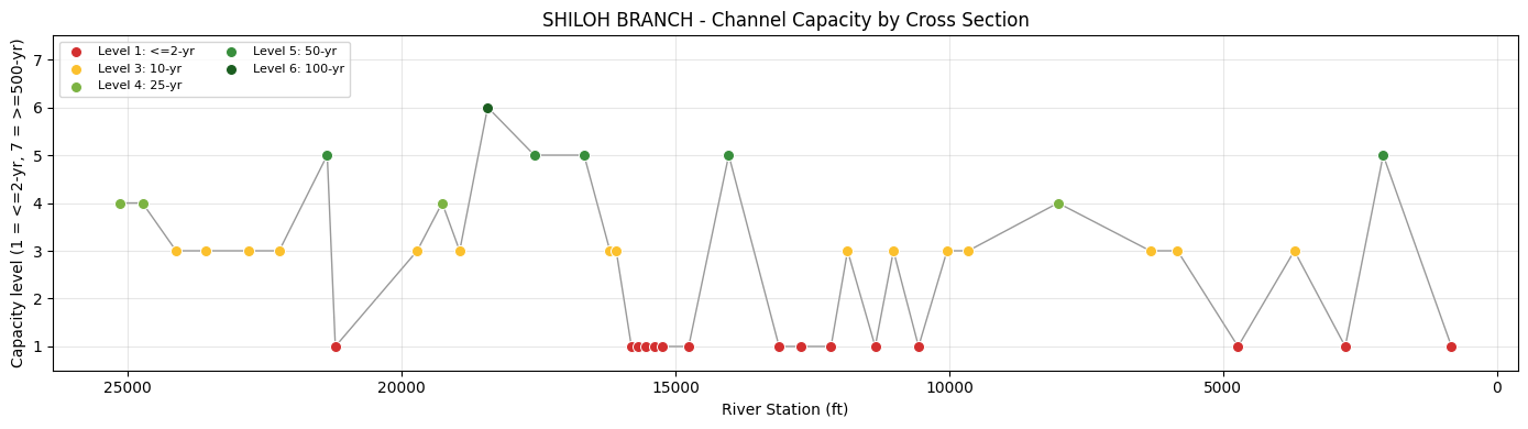
Step 3: Determine Channel Capacity
determine_capacity() tests storms from smallest (10P) to largest (0.2P) at each
cross section. The capacity level is the largest storm the channel can contain
without the WSE exceeding the controlling bank elevation.
capacity_df = HdfChannelCapacity.determine_capacity(
    bank_df, wse_df, storm_order=STORM_ORDER_BLE
)

print(f"Cross sections analyzed: {len(capacity_df)}")
print(f"\nCapacity distribution:")
for level in sorted(capacity_df['capacity_level'].unique()):
    count = (capacity_df['capacity_level'] == level).sum()
    category = LEVEL_TO_CATEGORY.get(level, 'Unknown')
    print(f"  Level {level} ({category}): {count} XS")

capacity_df[['RS', 'controlling_bank_elev', 'capacity_level',
             'capacity_category', 'last_contained_storm']].head(15)
Cross sections analyzed: 40

Capacity distribution:
  Level 1 (<=2-yr): 15 XS
  Level 3 (10-yr): 15 XS
  Level 4 (25-yr): 4 XS
  Level 5 (50-yr): 5 XS
  Level 6 (100-yr): 1 XS
| RS | controlling_bank_elev | capacity_level | capacity_category | last_contained_storm | |
|---|---|---|---|---|---|
| 0 | 25147 | 337.649994 | 4 | 25-yr | 4P |
| 1 | 24729 | 336.500000 | 4 | 25-yr | 4P |
| 2 | 24115 | 334.750000 | 3 | 10-yr | 10P |
| 3 | 23581 | 332.440002 | 3 | 10-yr | 10P |
| 4 | 22786 | 328.739990 | 3 | 10-yr | 10P |
| 5 | 22233 | 325.679993 | 3 | 10-yr | 10P |
| 6 | 21356 | 321.619995 | 5 | 50-yr | 2P |
| 7 | 21208 | 320.029999 | 1 | <=2-yr | None |
| 8 | 19714 | 313.519989 | 3 | 10-yr | 10P |
| 9 | 19258 | 310.820007 | 4 | 25-yr | 4P |
| 10 | 18938 | 309.250000 | 3 | 10-yr | 10P |
| 11 | 18427 | 306.619995 | 6 | 100-yr | 1P |
| 12 | 17575 | 300.890015 | 5 | 50-yr | 2P |
| 13 | 16667 | 298.640015 | 5 | 50-yr | 2P |
| 14 | 16195 | 295.160004 | 3 | 10-yr | 10P |
# Color-coded capacity level along the channel
fig, ax = plt.subplots(figsize=(14, 4))

rs_float = capacity_df['RS'].astype(float)
levels = capacity_df['capacity_level'].values

# Color map: red (lower capacity) to green (higher capacity)
capacity_colors = {
    1: '#D32F2F',  # Red - poor
    2: '#F57C00',  # Orange
    3: '#FBC02D',  # Yellow
    4: '#7CB342',  # Light green
    5: '#388E3C',  # Green
    6: '#1B5E20',  # Dark green
    7: '#0B3D0B',  # Deep green - highest tested capacity
}

plot_order = np.argsort(rs_float.values)
ax.plot(
    rs_float.iloc[plot_order],
    levels[plot_order],
    color='#555555',
    linewidth=1.0,
    alpha=0.6,
    zorder=1,
)

for level in sorted(set(levels)):
    mask = levels == level
    ax.scatter(
        rs_float[mask],
        levels[mask],
        s=52,
        color=capacity_colors.get(level, '#888888'),
        edgecolor='white',
        linewidth=0.7,
        label=f'Level {level}: {LEVEL_TO_CATEGORY[level]}',
        zorder=2,
    )

ax.legend(loc='upper left', fontsize=8, ncol=2)

ax.set_xlabel('River Station (ft)')
ax.set_ylabel('Capacity Level')
ax.set_title(f'{BLE_REACH_NAME} - Channel Capacity by Cross Section')
ax.set_ylim(0.5, 7.5)
ax.set_yticks(range(1, 8))
ax.invert_xaxis()
ax.grid(True, alpha=0.3)
plt.tight_layout()
plt.show()
Step 4: Segment Aggregation
segment_channel() groups cross sections into fixed-length segments (default: 0.25 mi)
and computes a weighted average capacity for each segment. The capacity is rounded DOWN
(conservative) to ensure the weakest areas in a segment are not masked.
segments_df = HdfChannelCapacity.segment_channel(
    capacity_df, segment_length=SEGMENT_LENGTH
)

print(f"Segments created: {len(segments_df)}")
print(f"Segment length: {SEGMENT_LENGTH:.0f} ft ({SEGMENT_LENGTH/5280:.2f} mi)")

segments_df
Segments created: 17
Segment length: 1320 ft (0.25 mi)
| River | Reach | river | reach | segment_id | segment_start_rs | segment_end_rs | start_distance | end_distance | segment_length_ft | segment_length_miles | weighted_capacity | capacity_level | capacity_category | system_capacity | channel_length | cross_section_count | xs_count | |
|---|---|---|---|---|---|---|---|---|---|---|---|---|---|---|---|---|---|---|
| 0 | SHILOH BRANCH | Reach-1 | SHILOH BRANCH | Reach-1 | 1 | 25147 | 24115 | 0.0 | 1320.0 | 1320.0 | 0.250000 | 3.66 | 3 | 10-yr | 10-yr | 1320.0 | 3 | 3 |
| 1 | SHILOH BRANCH | Reach-1 | SHILOH BRANCH | Reach-1 | 2 | 23581 | 22786 | 1320.0 | 2640.0 | 1320.0 | 0.250000 | 3.00 | 3 | 10-yr | 10-yr | 1320.0 | 2 | 2 |
| 2 | SHILOH BRANCH | Reach-1 | SHILOH BRANCH | Reach-1 | 3 | 22233 | 21208 | 2640.0 | 3960.0 | 1320.0 | 0.250000 | 1.93 | 1 | <=2-yr | <=2-yr | 1320.0 | 3 | 3 |
| 3 | SHILOH BRANCH | Reach-1 | SHILOH BRANCH | Reach-1 | 5 | 19714 | 18938 | 5280.0 | 6600.0 | 1320.0 | 0.250000 | 3.25 | 3 | 10-yr | 10-yr | 1320.0 | 3 | 3 |
| 4 | SHILOH BRANCH | Reach-1 | SHILOH BRANCH | Reach-1 | 6 | 18427 | 17575 | 6600.0 | 7920.0 | 1320.0 | 0.250000 | 5.48 | 5 | 50-yr | 50-yr | 1320.0 | 2 | 2 |
| 5 | SHILOH BRANCH | Reach-1 | SHILOH BRANCH | Reach-1 | 7 | 16667 | 16080 | 7920.0 | 9240.0 | 1320.0 | 0.250000 | 4.09 | 4 | 25-yr | 25-yr | 1320.0 | 3 | 3 |
| 6 | SHILOH BRANCH | Reach-1 | SHILOH BRANCH | Reach-1 | 8 | 15803 | 14758 | 9240.0 | 10560.0 | 1320.0 | 0.250000 | 1.00 | 1 | <=2-yr | <=2-yr | 1320.0 | 6 | 6 |
| 7 | SHILOH BRANCH | Reach-1 | SHILOH BRANCH | Reach-1 | 9 | 14026 | 14026 | 10560.0 | 11880.0 | 1320.0 | 0.250000 | 5.00 | 5 | 50-yr | 50-yr | 1320.0 | 1 | 1 |
| 8 | SHILOH BRANCH | Reach-1 | SHILOH BRANCH | Reach-1 | 10 | 13107 | 12159 | 11880.0 | 13200.0 | 1320.0 | 0.250000 | 1.00 | 1 | <=2-yr | <=2-yr | 1320.0 | 3 | 3 |
| 9 | SHILOH BRANCH | Reach-1 | SHILOH BRANCH | Reach-1 | 11 | 11857 | 11019 | 13200.0 | 14520.0 | 1320.0 | 0.250000 | 2.48 | 2 | 5-yr | 5-yr | 1320.0 | 3 | 3 |
| 10 | SHILOH BRANCH | Reach-1 | SHILOH BRANCH | Reach-1 | 12 | 10561 | 9655 | 14520.0 | 15840.0 | 1320.0 | 0.250000 | 2.59 | 2 | 5-yr | 5-yr | 1320.0 | 3 | 3 |
| 11 | SHILOH BRANCH | Reach-1 | SHILOH BRANCH | Reach-1 | 13 | 8015 | 8015 | 15840.0 | 17160.0 | 1320.0 | 0.250000 | 4.00 | 4 | 25-yr | 25-yr | 1320.0 | 1 | 1 |
| 12 | SHILOH BRANCH | Reach-1 | SHILOH BRANCH | Reach-1 | 15 | 6333 | 5834 | 18480.0 | 19800.0 | 1320.0 | 0.250000 | 3.00 | 3 | 10-yr | 10-yr | 1320.0 | 2 | 2 |
| 13 | SHILOH BRANCH | Reach-1 | SHILOH BRANCH | Reach-1 | 16 | 4729 | 4729 | 19800.0 | 21120.0 | 1320.0 | 0.250000 | 1.00 | 1 | <=2-yr | <=2-yr | 1320.0 | 1 | 1 |
| 14 | SHILOH BRANCH | Reach-1 | SHILOH BRANCH | Reach-1 | 17 | 3701 | 2772 | 21120.0 | 22440.0 | 1320.0 | 0.250000 | 2.15 | 2 | 5-yr | 5-yr | 1320.0 | 2 | 2 |
| 15 | SHILOH BRANCH | Reach-1 | SHILOH BRANCH | Reach-1 | 18 | 2079 | 2079 | 22440.0 | 23760.0 | 1320.0 | 0.250000 | 5.00 | 5 | 50-yr | 50-yr | 1320.0 | 1 | 1 |
| 16 | SHILOH BRANCH | Reach-1 | SHILOH BRANCH | Reach-1 | 19 | 832 | 832 | 23760.0 | 24315.0 | 555.0 | 0.105114 | 1.00 | 1 | <=2-yr | <=2-yr | 555.0 | 1 | 1 |
summary_df = HdfChannelCapacity.system_capacity_summary(segments_df)

print(f"Total channel length: {summary_df['channel_length_ft'].sum():,.0f} ft ")
print(f"                    = {summary_df['channel_length_ft'].sum()/5280:.2f} mi")
print()
summary_df
Total channel length: 21,675 ft
                    = 4.11 mi
| capacity_level | capacity_category | channel_length_ft | percent_of_total | xs_count | |
|---|---|---|---|---|---|
| 0 | 1 | <=2-yr | 5835.0 | 26.9 | 5 |
| 1 | 2 | 5-yr | 3960.0 | 18.3 | 3 |
| 2 | 3 | 10-yr | 5280.0 | 24.4 | 4 |
| 3 | 4 | 25-yr | 2640.0 | 12.2 | 2 |
| 4 | 5 | 50-yr | 3960.0 | 18.3 | 3 |
| 5 | 6 | 100-yr | 0.0 | 0.0 | 0 |
| 6 | 7 | >=500-yr | 0.0 | 0.0 | 0 |
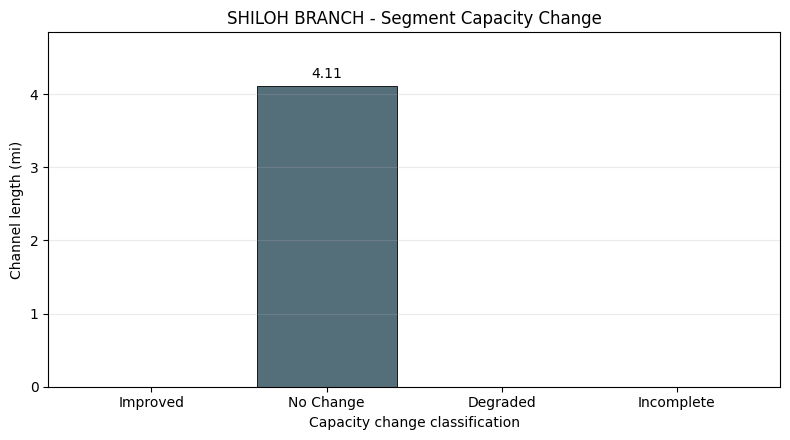
Step 5: Compare Existing and Proposed Conditions
compare_conditions() compares segment-level capacity between two analysis result dictionaries.
The public BLE example has one condition, so this cell uses the same real HDF-derived analysis for both
inputs as a no-change baseline. In project work, replace proposed_results with an analysis from the
proposed condition geometry/results HDFs.
existing_results = {
    'xs_capacity': capacity_df,
    'segments': segments_df,
    'summary': summary_df,
    'bank_elevations': bank_df,
    'max_wse': wse_df,
}
proposed_results = {
    'xs_capacity': capacity_df.copy(),
    'segments': segments_df.copy(),
    'summary': summary_df.copy(),
    'bank_elevations': bank_df.copy(),
    'max_wse': wse_df.copy(),
}

comparison_df = HdfChannelCapacity.compare_conditions(existing_results, proposed_results)
classification_lengths = (
    comparison_df.assign(channel_length_miles=segments_df['segment_length_ft'].values / 5280.0)
    .groupby('classification', as_index=False)['channel_length_miles'].sum()
)

print('Segment comparison counts:')
print(comparison_df['classification'].value_counts().to_string())
comparison_df[['River', 'Reach', 'segment_id', 'existing_level', 'proposed_level', 'level_change', 'classification']].head(10)
Segment comparison counts:
classification
No Change    17
| River | Reach | segment_id | existing_level | proposed_level | level_change | classification | |
|---|---|---|---|---|---|---|---|
| 0 | SHILOH BRANCH | Reach-1 | 1 | 3 | 3 | 0 | No Change |
| 1 | SHILOH BRANCH | Reach-1 | 2 | 3 | 3 | 0 | No Change |
| 2 | SHILOH BRANCH | Reach-1 | 3 | 1 | 1 | 0 | No Change |
| 3 | SHILOH BRANCH | Reach-1 | 5 | 3 | 3 | 0 | No Change |
| 4 | SHILOH BRANCH | Reach-1 | 6 | 5 | 5 | 0 | No Change |
| 5 | SHILOH BRANCH | Reach-1 | 7 | 4 | 4 | 0 | No Change |
| 6 | SHILOH BRANCH | Reach-1 | 8 | 1 | 1 | 0 | No Change |
| 7 | SHILOH BRANCH | Reach-1 | 9 | 5 | 5 | 0 | No Change |
| 8 | SHILOH BRANCH | Reach-1 | 10 | 1 | 1 | 0 | No Change |
| 9 | SHILOH BRANCH | Reach-1 | 11 | 2 | 2 | 0 | No Change |
fig, ax = plt.subplots(figsize=(7, 3.6))
class_order = ['Improved', 'No Change', 'Degraded', 'Incomplete']
class_colors = {
    'Improved': '#2E7D32',
    'No Change': '#546E7A',
    'Degraded': '#C62828',
    'Incomplete': '#6A1B9A',
}
plot_df = classification_lengths.copy()
plot_df['classification'] = pd.Categorical(plot_df['classification'], categories=class_order, ordered=True)
plot_df = plot_df.sort_values('classification')
bars = ax.barh(
    plot_df['classification'].astype(str),
    plot_df['channel_length_miles'],
    color=[class_colors[c] for c in plot_df['classification']],
    edgecolor='black',
    linewidth=0.6,
)
max_length = float(plot_df['channel_length_miles'].max())
ax.set_xlim(0, max_length * 1.18 if max_length > 0 else 1.0)
ax.bar_label(bars, labels=[f'{v:.2f} mi' for v in plot_df['channel_length_miles']], padding=4)
ax.set_title(f'{BLE_REACH_NAME} - Segment Capacity Change')
ax.set_xlabel('Total Channel Length (mi)')
ax.set_ylabel('Capacity Change Classification')
ax.grid(True, alpha=0.25, axis='x')
plt.tight_layout()
plt.show()
Key Takeaways
extract_bank_elevations()reads bank station elevations from the geometry HDF usingnp.interp()on station-elevation data.extract_steady_profile_wse()extracts individual steady-state profiles from a single plan HDF, preserving each AEP event as a separate column.determine_capacity()tests storms from smallest to largest, classifying each cross section into capacity levels 1-7.segment_channel()aggregates XS-level capacity into fixed-length segments with conservative (FLOOR) weighting.system_capacity_summary()produces the segment-weighted capacity distribution.compare_conditions()classifies segment-level capacity change as Improved, No Change, or Degraded.
Validation notes:
- This 1D steady reach does not rely on terrain or land-cover layers for the channel-capacity workflow.
- Missing .rasmap/CRS warnings are expected for this older BLE reach and are surfaced in the saved output.
- HdfResultsPlan may emit ERROR-level timestamp parsing logs when older steady HDF metadata stores simulation time as Unknown; the HEC-RAS run and profile extraction still complete successfully.
- The important evidence is that HEC-RAS runs the steady plan, produces geometry/result HDF files, and the profile WSE extraction returns coherent cross-section results.
For BLE models with a single plan and multiple steady profiles, use extract_steady_profile_wse() instead of extract_max_wse() (which is designed for multi-plan workflows where each AEP is a separate plan HDF).
References: - FEMA BLE program: https://www.fema.gov/flood-maps/products-tools/base-level-engineering