Steady Flow Calibration
from pathlib import Path
import logging

import matplotlib.pyplot as plt
from matplotlib.lines import Line2D
import numpy as np
import pandas as pd
from IPython.display import display

import ras_commander
from ras_commander import (
    HdfResultsPlan,
    RasCalibrate,
    RasCmdr,
    RasExamples,
    extract_steady_profile_observations,
    init_ras_project,
    make_steady_profile_calibration_points,
    make_xsec_mannings_apply_fn,
)
from ras_commander.geom import GeomCrossSection

logging.disable(logging.CRITICAL)
pd.options.display.max_columns = 20

print(f"ras-commander {ras_commander.__version__}")
ras-commander 0.98.0
Development Mode
When running this notebook from a source checkout instead of an installed package, start Jupyter from the repository root or add the repository root to PYTHONPATH before launching Jupyter. Generated example projects and run outputs are written under working/.
Steady Flow Calibration Helpers
This notebook demonstrates a steady-flow calibration workflow on a real HEC-RAS example project with many cross sections. The example starts from the default model, creates a realistic synthetic observed water-surface profile with a target point 0.2 ft above the default result, then adjusts a lower-reach Manning's n zone to recover that target while checking the residual pattern across the full reach.
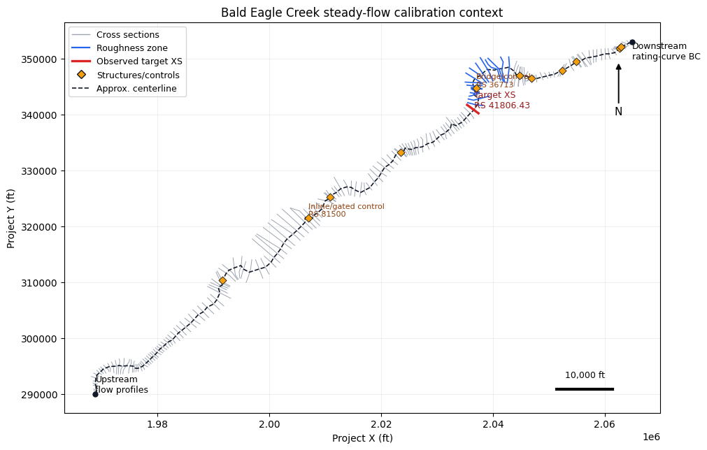
Model Context Checklist
Before calibrating, an engineer needs enough spatial and hydraulic context to know whether the adjustment is physically meaningful:
- Cross-section density and station order along the modeled reach.
- Upstream and downstream ends of the hydraulic reach, boundary-condition context, and structure/control locations.
- The steady-flow profile being calibrated and the downstream rating-curve boundary context.
- The target cross section, its lower-third reach location, and the roughness zone being adjusted.
- The spatial footprint of the WSE response, not just the target-point error.
The overview map below uses the model's GIS cut lines, river centerline approximation, structure/control station markers, upstream/downstream boundary labels, target cross section, and roughness-zone cross sections so the calibration control is visible before the residual plots. The map stays offline and reproducible by using model geometry rather than an external basemap service.
def find_repo_root(start):
    for candidate in [start, *start.parents]:
        if (candidate / "pyproject.toml").exists() and (candidate / "ras_commander").exists():
            return candidate
    return start


REPO_ROOT = find_repo_root(Path.cwd())
WORK_ROOT = REPO_ROOT / "working" / "steady_flow_calibration"
PROJECT_NAME = "Balde Eagle Creek"
PLAN_NUMBER = "02"
PROFILE_NAME = "100 year"
TARGET_FRACTION_DOWNSTREAM = 0.70
ZONE_XS_COUNT = 18
TARGET_WSE_OFFSET_FT = 0.20
SYNTHETIC_TRUTH_N = 0.055
CANDIDATE_N_VALUES = [0.045, 0.050, 0.055, 0.060, 0.070]
RAS_EXE = Path(r"C:\Program Files (x86)\HEC\HEC-RAS\7.0\Ras.exe")
ras_exe_arg = str(RAS_EXE) if RAS_EXE.exists() else "7.0"

WORK_ROOT.mkdir(parents=True, exist_ok=True)
project_path = RasExamples.extract_project(
    PROJECT_NAME,
    output_path=WORK_ROOT,
    suffix="clb496",
)
ras_project = init_ras_project(project_path, ras_exe_arg)

plan_overview = ras_project.plan_df[
    ["plan_number", "Plan Title", "flow_type", "Geom File", "Flow File"]
].copy()
display(plan_overview)
print(f"Repository root: {REPO_ROOT}")
print(f"Project path: {project_path}")
print(f"HEC-RAS executable: {ras_exe_arg}")
| plan_number | Plan Title | flow_type | Geom File | Flow File | |
|---|---|---|---|---|---|
| 0 | 01 | Unsteady with Bridges and Dam | Unsteady | 01 | 02 |
| 1 | 02 | Steady Flow Run | Steady | 01 | 02 |
Repository root: <workspace>
Project path: <workspace>\working\steady_flow_calibration\Balde Eagle Creek_clb496
HEC-RAS executable: <hec_ras_install>
compute_result = RasCmdr.compute_plan(
    PLAN_NUMBER,
    ras_object=ras_project,
    num_cores=1,
    verify=True,
    force_rerun=True,
)
assert compute_result, "HEC-RAS plan execution failed"

plan_hdf = project_path / f"{ras_project.project_name}.p{PLAN_NUMBER}.hdf"
assert plan_hdf.exists(), plan_hdf

profile_names = HdfResultsPlan.get_steady_profile_names(plan_hdf)
assert PROFILE_NAME in profile_names, profile_names
print(f"Computed default plan HDF: {plan_hdf}")
print(f"Steady profiles: {profile_names}")
Computed default plan HDF: <workspace>\working\steady_flow_calibration\Balde Eagle Creek_clb496\BaldEagle.p02.hdf
Steady profiles: ['.5 year', '1 year', '2 year', '5 year', '10 year', '25 year', '50 year', '100 year']
plan_row = ras_project.plan_df[
    ras_project.plan_df["plan_number"].astype(str).str.zfill(2).eq(PLAN_NUMBER)
].iloc[0]
geom_number = str(plan_row["Geom File"]).strip().zfill(2)
geom_path = project_path / f"{ras_project.project_name}.g{geom_number}"
assert geom_path.exists(), geom_path

xs_df = GeomCrossSection.get_cross_sections(geom_path)
natural_xs = xs_df[xs_df["Type"].eq(1)].copy()
natural_xs["station_numeric"] = pd.to_numeric(natural_xs["RS"], errors="coerce")
natural_xs = (
    natural_xs.dropna(subset=["station_numeric"])
    .sort_values("station_numeric", ascending=False)
    .reset_index(drop=True)
)
natural_xs["reach_fraction_downstream"] = natural_xs.index / (len(natural_xs) - 1)
assert len(natural_xs) >= 10

target_idx = round(TARGET_FRACTION_DOWNSTREAM * (len(natural_xs) - 1))
target_xs = natural_xs.iloc[target_idx]
TARGET_RIVER = target_xs["River"]
TARGET_REACH = target_xs["Reach"]
TARGET_STATION = str(target_xs["RS"])

target_fraction = float(target_xs["reach_fraction_downstream"])
assert target_fraction >= 2 / 3, target_fraction

zone_xs = natural_xs.iloc[target_idx : target_idx + ZONE_XS_COUNT].copy()
zone_stations = set(zone_xs["RS"].astype(str))

zone_summary_rows = []
for row in zone_xs.itertuples(index=False):
    mann = GeomCrossSection.get_mannings_n(
        geom_path,
        row.River,
        row.Reach,
        str(row.RS),
    )
    channel_n = mann.loc[mann["Subsection"].eq("Channel"), "n_value"].mean()
    zone_summary_rows.append(
        {
            "station": str(row.RS),
            "fraction_downstream": float(row.reach_fraction_downstream),
            "original_channel_n": float(channel_n),
        }
    )
zone_summary = pd.DataFrame(zone_summary_rows)

display(
    pd.DataFrame(
        [
            {
                "natural_xs_count": len(natural_xs),
                "target_river": TARGET_RIVER,
                "target_reach": TARGET_REACH,
                "target_station": TARGET_STATION,
                "target_fraction_downstream": target_fraction,
                "roughness_zone_xs_count": len(zone_xs),
                "zone_station_min": zone_summary["station"].iloc[-1],
                "zone_station_max": zone_summary["station"].iloc[0],
            }
        ]
    )
)
display(zone_summary.head(10))
| natural_xs_count | target_river | target_reach | target_station | target_fraction_downstream | roughness_zone_xs_count | zone_station_min | zone_station_max | |
|---|---|---|---|---|---|---|---|---|
| 0 | 178 | Bald Eagle | Loc Hav | 41806.43 | 0.700565 | 18 | 25960.70 | 41806.43 |
| station | fraction_downstream | original_channel_n | |
|---|---|---|---|
| 0 | 41806.43 | 0.700565 | 0.050 |
| 1 | 40526.85 | 0.706215 | 0.045 |
| 2 | 39499.37 | 0.711864 | 0.045 |
| 3 | 38446.87 | 0.717514 | 0.045 |
| 4 | 37962.54 | 0.723164 | 0.045 |
| 5 | 37385.23 | 0.728814 | 0.045 |
| 6 | 36769.88 | 0.734463 | 0.045 |
| 7 | 36663.76 | 0.740113 | 0.045 |
| 8 | 36339.56 | 0.745763 | 0.045 |
| 9 | 35648.50 | 0.751412 | 0.045 |
def make_xs_line_table(xs_coords):
    rows = []
    for (river, reach, station), group in xs_coords.groupby(["river", "reach", "RS"], sort=False):
        ordered = group.sort_values("station")
        rows.append(
            {
                "river": river,
                "reach": reach,
                "station": str(station),
                "x": ordered["x"].to_numpy(),
                "y": ordered["y"].to_numpy(),
                "x_mid": ordered["x"].mean(),
                "y_mid": ordered["y"].mean(),
            }
        )
    lines = pd.DataFrame(rows)
    station_lookup = natural_xs.set_index("RS")["reach_fraction_downstream"].to_dict()
    lines["fraction_downstream"] = lines["station"].map(station_lookup)
    return lines.sort_values("fraction_downstream")


xs_coords = GeomCrossSection.get_xs_coords(
    geom_path,
    river=TARGET_RIVER,
    reach=TARGET_REACH,
)
xs_lines = make_xs_line_table(xs_coords)
centerline = xs_lines.dropna(subset=["fraction_downstream"]).sort_values("fraction_downstream")
centerline_numeric = centerline.copy()
centerline_numeric["station_numeric"] = pd.to_numeric(centerline_numeric["station"], errors="coerce")
interp_source = centerline_numeric.dropna(subset=["station_numeric"]).sort_values("station_numeric")

structure_points = xs_df[
    (xs_df["Type"].ne(1))
    & (xs_df["River"].eq(TARGET_RIVER))
    & (xs_df["Reach"].eq(TARGET_REACH))
].copy()
structure_points["station_numeric"] = pd.to_numeric(structure_points["RS"], errors="coerce")
structure_points = structure_points.dropna(subset=["station_numeric"])
if not structure_points.empty and len(interp_source) >= 2:
    structure_points["x_mid"] = np.interp(
        structure_points["station_numeric"],
        interp_source["station_numeric"],
        interp_source["x_mid"],
    )
    structure_points["y_mid"] = np.interp(
        structure_points["station_numeric"],
        interp_source["station_numeric"],
        interp_source["y_mid"],
    )
else:
    structure_points = structure_points.assign(x_mid=np.nan, y_mid=np.nan).dropna(subset=["x_mid", "y_mid"])

def add_north_arrow(ax):
    ax.annotate(
        "N",
        xy=(0.93, 0.90),
        xytext=(0.93, 0.77),
        xycoords="axes fraction",
        ha="center",
        va="center",
        fontsize=11,
        arrowprops={"arrowstyle": "-|>", "lw": 1.4, "color": "black"},
    )


def add_scale_bar(ax, length=10000):
    xmin, xmax = ax.get_xlim()
    ymin, ymax = ax.get_ylim()
    x0 = xmax - length - 0.08 * (xmax - xmin)
    y0 = ymin + 0.06 * (ymax - ymin)
    ax.plot([x0, x0 + length], [y0, y0], color="black", linewidth=3)
    ax.text(
        x0 + length / 2,
        y0 + 0.025 * (ymax - ymin),
        f"{length:,.0f} ft",
        ha="center",
        va="bottom",
        fontsize=9,
    )


fig, ax = plt.subplots(figsize=(10, 7), constrained_layout=True)
for row in xs_lines.itertuples(index=False):
    color = "#9ca3af"
    linewidth = 0.7
    zorder = 1
    if row.station in zone_stations:
        color = "#2563eb"
        linewidth = 1.2
        zorder = 3
    if row.station == TARGET_STATION:
        color = "#dc2626"
        linewidth = 2.4
        zorder = 4
    ax.plot(row.x, row.y, color=color, linewidth=linewidth, zorder=zorder)

ax.plot(
    centerline["x_mid"],
    centerline["y_mid"],
    color="#111827",
    linestyle="--",
    linewidth=1.2,
    label="Approx. centerline",
    zorder=2,
)
upstream = centerline.iloc[0]
downstream = centerline.iloc[-1]
ax.scatter([upstream.x_mid, downstream.x_mid], [upstream.y_mid, downstream.y_mid], color="#111827", s=25, zorder=5)
ax.text(upstream.x_mid, upstream.y_mid, "Upstream\nflow profiles", fontsize=9, ha="left", va="bottom")
ax.text(downstream.x_mid, downstream.y_mid, "Downstream\nrating-curve BC", fontsize=9, ha="left", va="top")
if not structure_points.empty:
    ax.scatter(
        structure_points["x_mid"],
        structure_points["y_mid"],
        marker="D",
        s=32,
        facecolor="#f59e0b",
        edgecolor="#111827",
        linewidth=0.6,
        zorder=6,
    )
    label_structures = structure_points[
        structure_points["Type"].eq(5)
        | structure_points["station_numeric"].between(
            zone_xs["station_numeric"].min(),
            zone_xs["station_numeric"].max(),
        )
    ].copy()
    for row in label_structures.head(3).itertuples(index=False):
        label = "Inline/gated control" if int(row.Type) == 5 else "Bridge/control"
        ax.text(
            row.x_mid,
            row.y_mid,
            f"{label}\nRS {row.RS}",
            fontsize=8,
            color="#92400e",
            ha="left",
            va="bottom",
        )

target_line = xs_lines[xs_lines["station"].eq(TARGET_STATION)].iloc[0]
ax.text(
    target_line.x_mid,
    target_line.y_mid,
    f"Target XS\nRS {TARGET_STATION}",
    fontsize=9,
    color="#991b1b",
    ha="left",
    va="bottom",
)

handles = [
    Line2D([0], [0], color="#9ca3af", lw=1.0, label="Cross sections"),
    Line2D([0], [0], color="#2563eb", lw=1.6, label="Roughness zone"),
    Line2D([0], [0], color="#dc2626", lw=2.4, label="Observed target XS"),
    Line2D([0], [0], marker="D", color="white", markerfacecolor="#f59e0b", markeredgecolor="#111827", linestyle="None", label="Structures/controls"),
    Line2D([0], [0], color="#111827", lw=1.2, linestyle="--", label="Approx. centerline"),
]
ax.legend(handles=handles, loc="upper left", frameon=True, fontsize=9)
ax.set_aspect("equal", adjustable="box")
ax.set_xlabel("Project X (ft)")
ax.set_ylabel("Project Y (ft)")
ax.set_title("Bald Eagle Creek steady-flow calibration context")
ax.grid(True, alpha=0.2)
add_north_arrow(ax)
add_scale_bar(ax)
plt.show()
Synthetic Observed WSE Profile
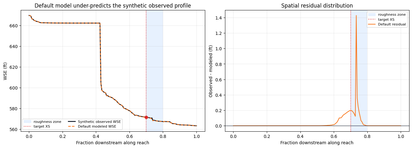
The default steady plan is treated as the model before calibration. To make the exercise realistic but repeatable, the synthetic observations represent a plausible rougher lower-reach condition rather than copying the default model output. The target observation is fixed at exactly 0.2 ft above the default computed WSE at a cross section in the lower third of the reach. The rest of the synthetic observed profile follows the spatial response from the same rougher-zone condition, scaled to honor that target offset.
def modeled_profile_from_hdf(hdf_path, profile_name):
    modeled = HdfResultsPlan.get_steady_wse(hdf_path, profile_name=profile_name)
    if "Profile" not in modeled.columns:
        modeled["Profile"] = profile_name
    modeled = modeled.rename(
        columns={
            "River": "river",
            "Reach": "reach",
            "Station": "station",
            "Profile": "profile",
            "WSE": "modeled",
        }
    )
    modeled["station"] = modeled["station"].astype(str).str.strip()
    return modeled[["river", "reach", "station", "profile", "modeled"]]


def comparison_from_modeled(observations, modeled, run_label):
    comparison = observations.merge(
        modeled[["station", "modeled"]],
        on="station",
        how="left",
        validate="one_to_one",
    )
    comparison["run"] = run_label
    comparison["residual"] = comparison["observed"] - comparison["modeled"]
    return comparison.sort_values("reach_fraction_downstream").reset_index(drop=True)


def rmse(values):
    return float(np.sqrt(np.mean(np.square(values))))


def add_zone_shading(ax):
    ax.axvspan(
        zone_xs["reach_fraction_downstream"].min(),
        zone_xs["reach_fraction_downstream"].max(),
        color="#dbeafe",
        alpha=0.65,
        label="roughness zone",
    )
    ax.axvline(target_fraction, color="#dc2626", linestyle=":", linewidth=1.4, label="target XS")


def plot_spatial_comparison(before, after=None, title="Steady WSE profile comparison"):
    fig, axes = plt.subplots(1, 2, figsize=(13, 4.6), constrained_layout=True)
    add_zone_shading(axes[0])
    axes[0].plot(
        before["reach_fraction_downstream"],
        before["observed"],
        color="#111827",
        linewidth=2.0,
        label="Synthetic observed WSE",
    )
    axes[0].plot(
        before["reach_fraction_downstream"],
        before["modeled"],
        color="#f97316",
        linestyle="--",
        linewidth=1.6,
        label="Default modeled WSE",
    )
    if after is not None:
        axes[0].plot(
            after["reach_fraction_downstream"],
            after["modeled"],
            color="#2563eb",
            linestyle="-.",
            linewidth=1.7,
            label="Calibrated modeled WSE",
        )
    target_obs = before.loc[before["is_target"]].iloc[0]
    axes[0].scatter(
        [target_obs["reach_fraction_downstream"]],
        [target_obs["observed"]],
        color="#dc2626",
        s=45,
        zorder=5,
    )
    axes[0].set_xlabel("Fraction downstream along reach")
    axes[0].set_ylabel("WSE (ft)")
    axes[0].set_title(title)
    axes[0].grid(True, alpha=0.25)
    axes[0].legend(fontsize=8, ncols=2)

    add_zone_shading(axes[1])
    axes[1].plot(
        before["reach_fraction_downstream"],
        before["residual"],
        color="#f97316",
        linewidth=1.5,
        label="Default residual",
    )
    if after is not None:
        axes[1].plot(
            after["reach_fraction_downstream"],
            after["residual"],
            color="#2563eb",
            linewidth=1.5,
            label="Calibrated residual",
        )
    axes[1].axhline(0, color="#111827", linewidth=0.8)
    axes[1].set_xlabel("Fraction downstream along reach")
    axes[1].set_ylabel("Observed - modeled (ft)")
    axes[1].set_title("Spatial residual distribution")
    axes[1].grid(True, alpha=0.25)
    axes[1].legend(fontsize=8)
    plt.show()
default_profile = extract_steady_profile_observations(plan_hdf, profiles=[PROFILE_NAME])
default_profile = default_profile.rename(columns={"observed": "default_model"})
default_profile = default_profile[
    (default_profile["river"].eq(TARGET_RIVER))
    & (default_profile["reach"].eq(TARGET_REACH))
].copy()

natural_lookup = natural_xs[
    ["RS", "station_numeric", "reach_fraction_downstream"]
].rename(columns={"RS": "station"})
natural_lookup["station"] = natural_lookup["station"].astype(str)
spatial_base = default_profile.merge(
    natural_lookup,
    on="station",
    how="inner",
    validate="one_to_one",
).sort_values("reach_fraction_downstream")

base_target_wse = float(
    spatial_base.loc[spatial_base["station"].eq(TARGET_STATION), "default_model"].iloc[0]
)
target_observed_wse = base_target_wse + TARGET_WSE_OFFSET_FT

target_observation = spatial_base.loc[spatial_base["station"].eq(TARGET_STATION)].copy()
target_observation["observed"] = target_observed_wse
calibration_points = make_steady_profile_calibration_points(
    target_observation[["river", "reach", "station", "profile", "observed"]],
    station_tolerance=0.01,
)

print(f"Default target WSE at RS {TARGET_STATION}: {base_target_wse:.3f} ft")
print(f"Synthetic observed target WSE: {target_observed_wse:.3f} ft")
print(f"Target offset: {target_observed_wse - base_target_wse:.3f} ft")
Default target WSE at RS 41806.43: 571.201 ft
Synthetic observed target WSE: 571.401 ft
Target offset: 0.200 ft
zone_mapping = {
    f"n_zone_{idx:02d}": {
        "river": TARGET_RIVER,
        "reach": TARGET_REACH,
        "station": str(row.RS),
        "subsection": "Channel",
    }
    for idx, row in enumerate(zone_xs.itertuples(index=False), start=1)
}
base_zone_apply_fn = make_xsec_mannings_apply_fn(zone_mapping, clone_geometry=True)


def apply_zone_n(plan_path, param_row, ras_object=None):
    expanded = pd.Series(
        {param_name: float(param_row["n_zone"]) for param_name in zone_mapping},
        dtype="object",
    )
    base_zone_apply_fn(plan_path, expanded, ras_object=ras_object)


truth_result = RasCalibrate.evaluate_single(
    PLAN_NUMBER,
    {"n_zone": SYNTHETIC_TRUTH_N},
    apply_zone_n,
    calibration_points,
    metric="rmse",
    num_cores=1,
    force_geompre=True,
    ras_object=ras_project,
)
assert truth_result["success"], truth_result

truth_modeled = modeled_profile_from_hdf(truth_result["hdf_path"], PROFILE_NAME).rename(
    columns={"modeled": "synthetic_truth_model"}
)
synthetic_profile = spatial_base.merge(
    truth_modeled[["station", "synthetic_truth_model"]],
    on="station",
    how="inner",
    validate="one_to_one",
)
synthetic_profile["truth_delta"] = (
    synthetic_profile["synthetic_truth_model"] - synthetic_profile["default_model"]
)
target_delta = float(
    synthetic_profile.loc[synthetic_profile["station"].eq(TARGET_STATION), "truth_delta"].iloc[0]
)
assert target_delta > 0, target_delta
observation_scale = TARGET_WSE_OFFSET_FT / target_delta
synthetic_profile["observed"] = (
    synthetic_profile["default_model"] + synthetic_profile["truth_delta"] * observation_scale
)
synthetic_profile["is_target"] = synthetic_profile["station"].eq(TARGET_STATION)
synthetic_profile["in_roughness_zone"] = synthetic_profile["station"].isin(zone_stations)

observed_target_check = float(
    synthetic_profile.loc[synthetic_profile["is_target"], "observed"].iloc[0]
)
assert abs(observed_target_check - target_observed_wse) < 1e-6

baseline_comparison = synthetic_profile.copy()
baseline_comparison["run"] = "default model"
baseline_comparison["modeled"] = baseline_comparison["default_model"]
baseline_comparison["residual"] = baseline_comparison["observed"] - baseline_comparison["modeled"]

observation_preview = synthetic_profile.loc[
    synthetic_profile["is_target"] | synthetic_profile["in_roughness_zone"],
    [
        "river",
        "reach",
        "station",
        "profile",
        "reach_fraction_downstream",
        "default_model",
        "observed",
        "truth_delta",
        "is_target",
    ],
].head(12)

display(observation_preview)
print(f"Synthetic observation scale factor: {observation_scale:.4f}")
print(f"Default spatial RMSE: {rmse(baseline_comparison['residual']):.4f} ft")
print(
    "Default target residual: "
    f"{baseline_comparison.loc[baseline_comparison['is_target'], 'residual'].iloc[0]:.4f} ft"
)
| river | reach | station | profile | reach_fraction_downstream | default_model | observed | truth_delta | is_target | |
|---|---|---|---|---|---|---|---|---|---|
| 124 | Bald Eagle | Loc Hav | 41806.43 | 100 year | 0.700565 | 571.201294 | 571.401294 | 0.108948 | True |
| 125 | Bald Eagle | Loc Hav | 40526.85 | 100 year | 0.706215 | 571.089111 | 571.285750 | 0.107117 | False |
| 126 | Bald Eagle | Loc Hav | 39499.37 | 100 year | 0.711864 | 570.967468 | 571.154247 | 0.101746 | False |
| 127 | Bald Eagle | Loc Hav | 38446.87 | 100 year | 0.717514 | 570.724243 | 570.894999 | 0.093018 | False |
| 128 | Bald Eagle | Loc Hav | 37962.54 | 100 year | 0.723164 | 570.585815 | 570.736740 | 0.082214 | False |
| 129 | Bald Eagle | Loc Hav | 37385.23 | 100 year | 0.728814 | 570.362610 | 570.484627 | 0.066467 | False |
| 130 | Bald Eagle | Loc Hav | 36769.88 | 100 year | 0.734463 | 569.298462 | 570.725241 | 0.777222 | False |
| 131 | Bald Eagle | Loc Hav | 36663.76 | 100 year | 0.740113 | 567.896729 | 568.253367 | 0.194275 | False |
| 132 | Bald Eagle | Loc Hav | 36339.56 | 100 year | 0.745763 | 568.362854 | 568.611593 | 0.135498 | False |
| 133 | Bald Eagle | Loc Hav | 35648.50 | 100 year | 0.751412 | 568.104431 | 568.283367 | 0.097473 | False |
| 134 | Bald Eagle | Loc Hav | 35072.37 | 100 year | 0.757062 | 567.922241 | 568.046387 | 0.067627 | False |
| 135 | Bald Eagle | Loc Hav | 34098.93 | 100 year | 0.762712 | 567.787537 | 567.853307 | 0.035828 | False |
Synthetic observation scale factor: 1.8357
Default spatial RMSE: 0.1241 ft
Default target residual: 0.2000 ft
plot_spatial_comparison(
    baseline_comparison,
    title="Default model under-predicts the synthetic observed profile",
)
Manning's n Calibration
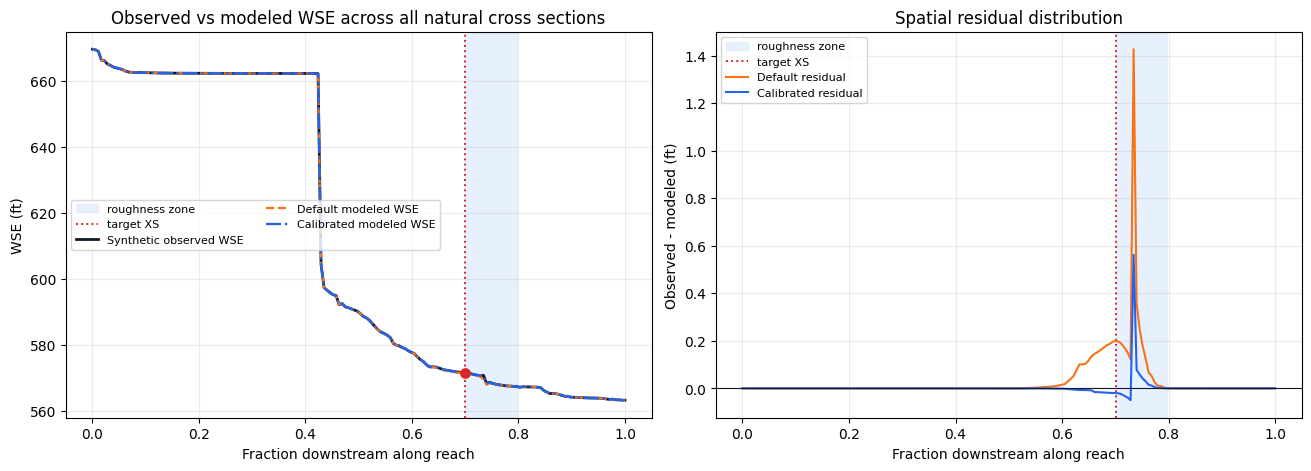
The calibration parameter is a single channel roughness value applied to a contiguous lower-reach zone. That mirrors a common steady-flow calibration decision: define a hydraulically coherent roughness zone, evaluate a small range of Manning's n values, and select the value that reduces the target residual while checking that residuals across the rest of the reach improve rather than merely hiding a local error.
calibration_rows = []
calibration_results = {}
for n_zone in CANDIDATE_N_VALUES:
    result = RasCalibrate.evaluate_single(
        PLAN_NUMBER,
        {"n_zone": n_zone},
        apply_zone_n,
        calibration_points,
        metric="rmse",
        num_cores=1,
        force_geompre=True,
        ras_object=ras_project,
    )
    modeled_target = result["point_results"][0]["modeled"] if result["point_results"] else np.nan
    calibration_rows.append(
        {
            "n_zone": n_zone,
            "success": result["success"],
            "target_observed_ft": target_observed_wse,
            "target_modeled_ft": modeled_target,
            "target_residual_ft": target_observed_wse - modeled_target,
            "target_rmse_ft": result["overall_objective"],
        }
    )
    calibration_results[n_zone] = result

calibration_summary = pd.DataFrame(calibration_rows)
min_target_rmse = calibration_summary["target_rmse_ft"].min()
RMSE_TIE_TOLERANCE_FT = 0.001
near_best = calibration_summary[
    calibration_summary["target_rmse_ft"] <= min_target_rmse + RMSE_TIE_TOLERANCE_FT
]
# Conservative tie-break: use the lowest n value that is indistinguishable at the target.
best_n = float(near_best.sort_values("n_zone").iloc[0]["n_zone"])
calibration_summary = calibration_summary.sort_values(["target_rmse_ft", "n_zone"]).reset_index(drop=True)

final_result = RasCalibrate.evaluate_single(
    PLAN_NUMBER,
    {"n_zone": best_n},
    apply_zone_n,
    calibration_points,
    metric="rmse",
    num_cores=1,
    force_geompre=True,
    ras_object=ras_project,
)
assert final_result["success"], final_result

final_modeled = modeled_profile_from_hdf(final_result["hdf_path"], PROFILE_NAME)
calibrated_comparison = comparison_from_modeled(
    synthetic_profile,
    final_modeled,
    f"calibrated n={best_n:.3f}",
)

display(calibration_summary)
print(f"Selected calibrated Manning's n: {best_n:.3f}")
print(f"Original zone channel n median: {zone_summary['original_channel_n'].median():.3f}")
print(
    "Tie-break rule: when candidates are within "
    f"{RMSE_TIE_TOLERANCE_FT:.3f} ft target RMSE, choose the lower n "
    "to avoid over-roughening."
)
| n_zone | success | target_observed_ft | target_modeled_ft | target_residual_ft | target_rmse_ft | |
|---|---|---|---|---|---|---|
| 0 | 0.060 | True | 571.401294 | 571.421204 | -0.019910 | 0.019910 |
| 1 | 0.050 | True | 571.401294 | 571.353149 | 0.048145 | 0.048145 |
| 2 | 0.055 | True | 571.401294 | 571.310242 | 0.091052 | 0.091052 |
| 3 | 0.070 | True | 571.401294 | 571.598389 | -0.197095 | 0.197095 |
| 4 | 0.045 | True | 571.401294 | 571.195374 | 0.205920 | 0.205920 |
Selected calibrated Manning's n: 0.060
Original zone channel n median: 0.045
Tie-break rule: when candidates are within 0.001 ft target RMSE, choose the lower n to avoid over-roughening.
plot_spatial_comparison(
baseline_comparison,
calibrated_comparison,
title="Observed vs modeled WSE across all natural cross sections",
)
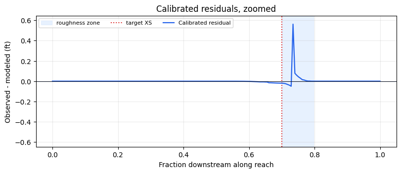
fig, ax = plt.subplots(figsize=(8, 3.4), constrained_layout=True)
add_zone_shading(ax)
ax.plot(
calibrated_comparison["reach_fraction_downstream"],
calibrated_comparison["residual"],
color="#2563eb",
linewidth=1.6,
label="Calibrated residual",
)
ax.axhline(0, color="#111827", linewidth=0.8)
zoom_limit = max(0.03, float(calibrated_comparison["residual"].abs().max()) * 1.15)
ax.set_ylim(-zoom_limit, zoom_limit)
ax.set_xlabel("Fraction downstream along reach")
ax.set_ylabel("Observed - modeled (ft)")
ax.set_title("Calibrated residuals, zoomed")
ax.grid(True, alpha=0.25)
ax.legend(fontsize=8, ncols=3)
plt.show()
metric_summary = pd.DataFrame(
[
{
"run": "default model",
"target_rmse_ft": abs(
baseline_comparison.loc[baseline_comparison["is_target"], "residual"].iloc[0]
),
"spatial_rmse_ft": rmse(baseline_comparison["residual"]),
"spatial_max_abs_residual_ft": float(baseline_comparison["residual"].abs().max()),
},
{
"run": f"calibrated n={best_n:.3f}",
"target_rmse_ft": abs(
calibrated_comparison.loc[calibrated_comparison["is_target"], "residual"].iloc[0]
),
"spatial_rmse_ft": rmse(calibrated_comparison["residual"]),
"spatial_max_abs_residual_ft": float(calibrated_comparison["residual"].abs().max()),
},
]
)
target_residual_table = pd.concat(
[
baseline_comparison.loc[baseline_comparison["is_target"]].assign(run="default model"),
calibrated_comparison.loc[calibrated_comparison["is_target"]],
],
ignore_index=True,
)[["run", "station", "observed", "modeled", "residual"]]
display(metric_summary)
display(target_residual_table)
print(
"Target RMSE improved from "
f"{metric_summary.loc[0, 'target_rmse_ft']:.4f} ft to "
f"{metric_summary.loc[1, 'target_rmse_ft']:.4f} ft"
)
print(
"Spatial RMSE improved from "
f"{metric_summary.loc[0, 'spatial_rmse_ft']:.4f} ft to "
f"{metric_summary.loc[1, 'spatial_rmse_ft']:.4f} ft"
)
| run | target_rmse_ft | spatial_rmse_ft | spatial_max_abs_residual_ft | |
|---|---|---|---|---|
| 0 | default model | 0.20000 | 0.124060 | 1.426779 |
| 1 | calibrated n=0.060 | 0.01991 | 0.043509 | 0.561788 |
| run | station | observed | modeled | residual | |
|---|---|---|---|---|---|
| 0 | default model | 41806.43 | 571.401294 | 571.201294 | 0.20000 |
| 1 | calibrated n=0.060 | 41806.43 | 571.401294 | 571.421204 | -0.01991 |
Target RMSE improved from 0.2000 ft to 0.0199 ft
Spatial RMSE improved from 0.1241 ft to 0.0435 ft
assert len(natural_xs) >= 10
assert target_fraction >= 2 / 3
assert abs(target_observed_wse - base_target_wse - TARGET_WSE_OFFSET_FT) < 1e-9
assert best_n > zone_summary["original_channel_n"].median()
assert metric_summary.loc[1, "target_rmse_ft"] < 0.02
assert metric_summary.loc[1, "spatial_rmse_ft"] < metric_summary.loc[0, "spatial_rmse_ft"]

print("Executed steady-flow calibration workflow against a 178-XS RasExamples project.")
print(f"Project: {PROJECT_NAME}")
print(f"Plan/profile: {PLAN_NUMBER} / {PROFILE_NAME}")
print(f"Target: {TARGET_RIVER} / {TARGET_REACH} / RS {TARGET_STATION}")
print(f"Calibrated lower-reach channel n: {best_n:.3f}")
print(f"Final plan HDF: {final_result['hdf_path']}")
Executed steady-flow calibration workflow against a 178-XS RasExamples project.
Project: Balde Eagle Creek
Plan/profile: 02 / 100 year
Target: Bald Eagle / Loc Hav / RS 41806.43
Calibrated lower-reach channel n: 0.060
Final plan HDF: <workspace>\working\steady_flow_calibration\Balde Eagle Creek_clb496\BaldEagle.p02.hdf