HECRASController Profiles
# =============================================================================
# DEVELOPMENT MODE TOGGLE
# =============================================================================
USE_LOCAL_SOURCE = False  # <-- TOGGLE THIS

import sys
from pathlib import Path

if USE_LOCAL_SOURCE:
    local_path = str(Path.cwd().parent)
    if local_path not in sys.path:
        sys.path.insert(0, local_path)
    print(f"LOCAL SOURCE MODE: Loading from {local_path}/ras_commander")
else:
    print("PIP PACKAGE MODE: Loading installed ras-commander")

# Import ras-commander
from ras_commander import RasCmdr, RasControl, RasExamples, RasPlan, init_ras_project, ras

# Additional imports for this notebook
import os
import pandas as pd
import matplotlib.pyplot as plt
import matplotlib.dates as mdates
import numpy as np
from IPython import display

# Verify which version loaded
import ras_commander
print(f"Loaded: {ras_commander.__file__}")
PIP PACKAGE MODE: Loading installed ras-commander


Loaded: G:\GH\ras-commander-pr-docs\ras_commander\__init__.py
Prerequisites
Before running this notebook, ensure you have:
- ras-commander installed:
pip install ras-commander - Python 3.10+: Check with
python --version - HEC-RAS 5.x or earlier: COM interface requires legacy versions
- pywin32:
pip install pywin32
What You'll Learn
This notebook demonstrates legacy COM-based automation using RasControl:
- HECRASController: COM interface for HEC-RAS 3.x-5.x
- Steady Flow Results: Extract profiles from steady flow runs
- Unsteady Flow Results: Time series data from unsteady runs
- Comparison Across Versions: Run same project in multiple HEC-RAS versions
Related Notebooks
- 110_single_plan_execution.ipynb - Command-line execution with
RasCmdr(HEC-RAS 5.0+) - 120_automating_ras_with_win32com.ipynb - GUI automation
Critical Information: HEC-RAS Version Compatibility
RasControl (COM interface): - Supported: HEC-RAS 3.x, 4.x, 5.x - NOT Supported: HEC-RAS 6.x+ (no COM interface)
Command-line execution (RasCmdr.compute_plan):
- Supported: HEC-RAS 5.0+
- HEC-RAS 5.x: ras-commander sets the requested plan current and uses the project-first -c layout
- HEC-RAS 6.0+: ras-commander passes -c, the project, and the explicit plan
- Result APIs: HDF-based features still depend on the files produced by that HEC-RAS release
- NOT Supported: HEC-RAS 3.x-4.x (use RasControl)
When to Use RasControl
Use RasControl when: 1. Working with HEC-RAS 3.x-4.x, or when a 5.x workflow specifically needs COM result access 2. Need to compare results across HEC-RAS versions 3. Legacy systems require COM interface 4. Accessing features not yet in modern API
Use RasCmdr.compute_plan() when:
1. Executing plans with HEC-RAS 5.0 or later
2. New projects (start with latest HEC-RAS)
3. Production workflows (faster, more reliable)
4. HDF-based results are available for the selected release
For unattended execution, accept the TCU for the exact installed release and current Windows user before launching. RasTcu.status(ras_object=ras) is a read-only check; an unaccepted release now fails fast instead of blocking behind a hidden modal dialog.
Migration Path: Legacy → Modern
Step 1: Upgrade project to HEC-RAS 6.x
Step 2: Replace RasControl with RasCmdr
# ❌ Legacy (RasControl - HEC-RAS 5.x)
RasControl.compute_plan("01")
df = RasControl.get_steady_results("01")

# ✅ Modern (RasCmdr - HEC-RAS 6.x)
RasCmdr.compute_plan("01")
hdf = HdfResultsPlan(ras.plan_df.loc[0, 'hdf_path'])
df = hdf.get_wse_dataframe()
Verification: COM-Based Execution
Success Criteria: - HEC-RAS opens automatically (COM instantiation) - Project loads in HEC-RAS window - Plan computes without errors - Results extracted to DataFrame
Visual Inspection: 1. HEC-RAS GUI window should appear 2. Project name visible in title bar 3. Computation messages shown in HEC-RAS window 4. Results available in HEC-RAS viewer
Troubleshooting COM Errors:
Error 1: "COM object not found"
# Verify HEC-RAS is registered
import win32com.client

try:
    ras_ctrl = win32com.client.Dispatch("RAS66.HECRASController")
    print("[OK] HEC-RAS COM registered")
except Exception as e:
    print(f"[ERROR] COM registration issue: {e}")
    print("Solution: Reinstall HEC-RAS or run as Administrator")
Error 2: "Project won't open"
# Check project file path
from pathlib import Path

prj_file = Path(project_folder) / "project.prj"
assert prj_file.exists(), f"Project file not found: {prj_file}"
print(f"[OK] Project file exists: {prj_file}")
Error 3: "Results not extracting"
# Verify plan computed successfully
# Check HEC-RAS GUI for computation messages
# Look for "Run completed successfully"
Understanding COM Output Structure
RasControl returns results in different formats than modern API:
Steady Flow (RasControl.get_steady_results):
# Returns DataFrame with columns:
# - river_id
# - reach_id
# - node_id
# - profile (profile number/name)
# - wse (water surface elevation)
# - velocity
# - etc.
Unsteady Flow (RasControl.get_unsteady_results):
# Returns DataFrame with columns:
# - river_id
# - reach_id
# - node_id
# - datetime (parsed from computation)
# - wse
# - velocity
# - etc.
Parameters
Configure these values to customize the notebook for your project.
# =============================================================================
# PARAMETERS - Edit these to customize the notebook
# =============================================================================
from pathlib import Path

# Project Configuration
PROJECT_NAME = "Muncie"           # Example project to extract
RAS_VERSION = "7.0"               # HEC-RAS version (5.0.5, 6.0, 6.6, 7.0, etc.)

print(f"Project: {PROJECT_NAME}")
print(f"HEC-RAS Version: {RAS_VERSION}")
Project: Muncie
HEC-RAS Version: 7.0
Working with Legacy HEC-RAS Using RasControl
This notebook demonstrates RasControl, which provides a ras-commander style API for legacy HEC-RAS versions (3.x-4.x) using the HECRASController COM interface.
What is RasControl?
RasControl wraps the HECRASController COM API with ras-commander conventions:
- ✅ Use plan numbers -
RasControl.run_plan("02")not file paths - ✅ Integrated with ras object - Works with
init_ras_project() - ✅ Steady AND unsteady - Extract profiles and time series
- ✅ Auto-sets current plan - Just pass the plan number!
- ✅ No COM complexity - Clean public API
When to Use RasControl
| Use RasControl | Use HDF Methods |
|---|---|
| HEC-RAS 3.1, 4.1 | HEC-RAS 6.0+ |
| No HDF support | Modern versions |
| Legacy models | 2D mesh data |
| Version migration | Better performance |
Supported Versions
3.0, 3.1, 4.0, 4.1, 5.0-5.0.7, 6.0-6.7 Beta
Accepts: "4.1", "41", "5.0.6", "506", "6.6", "66", etc.
Setup
# ============================================================================
# PLOTTING CONFIGURATION
# ============================================================================

# Set better default plotting parameters
plt.rcParams['figure.dpi'] = 100
plt.rcParams['savefig.dpi'] = 300
plt.rcParams['font.size'] = 10
plt.rcParams['axes.labelsize'] = 11
plt.rcParams['axes.titlesize'] = 12
plt.rcParams['legend.fontsize'] = 9
plt.rcParams['xtick.labelsize'] = 9
plt.rcParams['ytick.labelsize'] = 9

import numpy as np  # Add if not already imported

print("✓ Plotting configuration loaded")
✓ Plotting configuration loaded
Extract and Initialize Project
# Extract example project
project_path = RasExamples.extract_project("Balde Eagle Creek", suffix="17")

# Initialize project with HEC-RAS 6.6
init_ras_project(project_path, RAS_VERSION)

print(f"✓ Project initialized: {project_path}")
2026-07-07 18:15:20 - ras_commander.RasExamples - INFO - Successfully extracted project 'Balde Eagle Creek' to example_projects\Balde Eagle Creek_17


2026-07-07 18:15:21 - ras_commander.RasPrj - WARNING - Could not resolve project CRS for Balde Eagle Creek_17


2026-07-07 18:15:21 - ras_commander.RasPrj - INFO - ras-commander v0.98.2 | An open-source project of CLB Engineering Corporation (https://clbengineering.com/) | Docs: https://rascommander.info | GitHub: https://github.com/gpt-cmdr/ras-commander


2026-07-07 18:15:21 - ras_commander.RasPrj - INFO - Project initialized: BaldEagle


2026-07-07 18:15:21 - ras_commander.RasPrj - INFO - Using HEC-RAS version 7.0


2026-07-07 18:15:21 - ras_commander.RasPrj - INFO -
═══════════════════════════════════════════════════════════════════════
ras-commander | HEC-RAS Automation Library
Docs: https://rascommander.info/
Repo: https://github.com/gpt-cmdr/ras-commander
LLM agents: https://rascommander.info/llms.txt
═══════════════════════════════════════════════════════════════════════

PROJECT DATAFRAMES (single source of truth — use these, not file globbing):
  ras.plan_df        Plans, HDF paths, geometry/flow associations
  ras.geom_df        Geometry files and HDF preprocessor paths
  ras.flow_df        Steady flow files
  ras.unsteady_df    Unsteady flow files and configurations
  ras.boundaries_df  Boundary conditions (type, name, location)
  ras.results_df     Lightweight HDF results summaries
  ras.rasmap_df      RASMapper layers, terrain, land cover paths

KEY APIS (static classes — call directly, never instantiate):
  Execution:    RasCmdr.compute_plan() / compute_parallel() / compute_test_mode()
  Plan Files:   RasPlan.clone_plan() / clone_geom() / set_geom()
  Unsteady:     RasUnsteady — IC/BC management, gate openings, precipitation
  Geometry:     GeomCrossSection, GeomBridge, GeomStorage, GeomLateral, GeomMesh
  HDF Results:  HdfResultsPlan.get_wse() / get_compute_messages()
                HdfResultsMesh.get_mesh_max_ws() / get_mesh_cells_timeseries()
                HdfMesh.get_mesh_cell_points()
  QA/QC:        RasCheck.run_check() / RasFixit (geometry repair)
  DSS:          RasDss.get_timeseries() / check_pathname()
  USGS:         UsgsGaugeSpatial, GaugeMatcher, RasUsgsBoundaryGeneration
  Precipitation: StormGenerator, Atlas14Storm, PrecipAorc, Atlas14Variance
  Terrain:      RasTerrain.create_terrain_hdf() / RasTerrainMod

MULTI-PROJECT: Pass ras_object= to all API calls when using local RasPrj instances.

EXAMPLES: 100+ notebooks in examples/ (100s=execution, 200s=geometry, 300s=unsteady,
  400s=HDF results, 500s=remote, 800s=QA/QC, 900s=data integration).
  Review relevant notebooks before assembling new workflows.

PLATFORM: Most HEC-RAS operations require Windows. Linux/Wine support for
  headless execution, data access, geometry modification, and preprocessing
  is available via RasProcess (HEC-RAS 6.6+). See ras_commander/RasProcess.py.
  Remote distributed execution: ras_commander/remote/ (PsExec, Docker, SSH, cloud).
═══════════════════════════════════════════════════════════════════════


✓ Project initialized: G:\GH\ras-commander-pr-docs\examples\example_projects\Balde Eagle Creek_17
| plan_number | unsteady_number | geometry_number | Plan Title | Program Version | Short Identifier | Simulation Date | Computation Interval | Mapping Interval | Run HTab | ... | PS Cores | DSS File | Friction Slope Method | HDF_Results_Path | Geom File | Geom Path | Flow File | Flow Path | full_path | flow_type | |
|---|---|---|---|---|---|---|---|---|---|---|---|---|---|---|---|---|---|---|---|---|---|
| 0 | 01 | 02 | 01 | Unsteady with Bridges and Dam | 5.00 | UnsteadyFlow | 18FEB1999,0000,24FEB1999,0500 | 2MIN | 1HOUR | 1 | ... | None | dss | 2 | None | 01 | G:\GH\ras-commander-pr-docs\examples\example_p... | 02 | G:\GH\ras-commander-pr-docs\examples\example_p... | G:\GH\ras-commander-pr-docs\examples\example_p... | Unsteady |
| 1 | 02 | NaN | 01 | Steady Flow Run | NaN | SteadyRun | 02/18/1999,0000,02/24/1999,0500 | 2MIN | NaN | 1 | ... | None | dss | 1 | None | 01 | G:\GH\ras-commander-pr-docs\examples\example_p... | 02 | G:\GH\ras-commander-pr-docs\examples\example_p... | G:\GH\ras-commander-pr-docs\examples\example_p... | Steady |
2 rows × 32 columns
Part 1: Steady State (Plan 02)
Extract steady profiles. Note: run_plan() automatically sets Plan 02 as current!
# =============================================================================
# Run Plan 02 (Steady Flow)
# =============================================================================
# Must run the plan before extracting results
print("Running Plan 02 (Steady Flow)...")
RasCmdr.compute_plan("02", num_cores=2)
print("✓ Plan 02 completed")
Running Plan 02 (Steady Flow)...


2026-07-07 18:15:21 - ras_commander.RasUtils - INFO - Successfully updated file: BaldEagle.p02


2026-07-07 18:15:21 - ras_commander.RasCmdr - INFO - Set number of cores to 2 for plan: 02


2026-07-07 18:15:21 - ras_commander.RasCmdr - INFO - Running Ras.exe with -c command line flag for plan 02


2026-07-07 18:15:25 - ras_commander.RasCmdr - INFO - HEC-RAS execution completed for plan 02 in 4.17 seconds


✓ Plan 02 completed
Extracting Computation Messages (Steady Flow)
After running the plan, we can extract detailed computation messages using RasControl.get_comp_msgs(). This method:
- Reads from .comp_msgs.txt or .computeMsgs.txt files (version-dependent)
- Falls back to HDF extraction if .txt files not available
- Returns detailed information about the computation process
# Extract computation messages for steady flow Plan 02
print("="*80)
print("COMPUTATION MESSAGES - Plan 02 (Steady Flow)")
print("="*80)

msgs_steady = RasControl.get_comp_msgs("02")

if msgs_steady:
    print(f"\nExtracted {len(msgs_steady)} characters of computation messages\n")

    # Display first 800 characters
    print("Computation messages (first 800 characters):")
    print("-" * 80)
    print(msgs_steady[:800])

    if len(msgs_steady) > 800:
        print("\n... (truncated) ...")
else:
    print("No computation messages available for Plan 02")

print("\n" + "="*80)
================================================================================
COMPUTATION MESSAGES - Plan 02 (Steady Flow)
================================================================================
No computation messages available for Plan 02

================================================================================
# Extract steady results (auto-sets Plan 02 as current)
df_steady = RasControl.get_steady_results("02")

print(f"Rows: {len(df_steady)}")
print(f"Profiles: {df_steady['profile'].nunique()}")
print(f"XS: {df_steady['node_id'].nunique()}")
df_steady.head(10)
Rows: 1424
Profiles: 8
XS: 178
| river | reach | node_id | profile | wsel | min_ch_el | velocity | flow | froude | energy | max_depth | |
|---|---|---|---|---|---|---|---|---|---|---|---|
| 0 | Bald Eagle | Loc Hav | 138154.4 | .5 year | 660.588928 | 656.299988 | 3.657029 | 1.177402 | 0.363896 | 660.775635 | 4.288940 |
| 1 | Bald Eagle | Loc Hav | 138154.4 | 1 year | 661.432068 | 656.299988 | 3.888445 | 1.654405 | 0.358103 | 661.629578 | 5.132080 |
| 2 | Bald Eagle | Loc Hav | 138154.4 | 2 year | 662.602600 | 656.299988 | 4.519829 | 2.233629 | 0.365692 | 662.858398 | 6.302612 |
| 3 | Bald Eagle | Loc Hav | 138154.4 | 5 year | 664.673218 | 656.299988 | 5.791487 | 3.227041 | 0.396946 | 665.082153 | 8.373230 |
| 4 | Bald Eagle | Loc Hav | 138154.4 | 10 year | 666.190918 | 656.299988 | 6.828511 | 3.987156 | 0.426974 | 666.755981 | 9.890930 |
| 5 | Bald Eagle | Loc Hav | 138154.4 | 25 year | 667.459351 | 656.299988 | 7.730279 | 4.592227 | 0.449943 | 668.181274 | 11.159363 |
| 6 | Bald Eagle | Loc Hav | 138154.4 | 50 year | 668.543640 | 656.299988 | 8.564765 | 5.127679 | 0.471433 | 669.427612 | 12.243652 |
| 7 | Bald Eagle | Loc Hav | 138154.4 | 100 year | 669.521484 | 656.299988 | 9.320695 | 5.608300 | 0.490210 | 670.566101 | 13.221497 |
| 8 | Bald Eagle | Loc Hav | 137690.8 | .5 year | 659.914612 | 653.729980 | 3.339625 | 0.703524 | 0.282183 | 660.072205 | 6.184631 |
| 9 | Bald Eagle | Loc Hav | 137690.8 | 1 year | 660.849548 | 653.729980 | 3.501968 | 1.028502 | 0.274149 | 661.000366 | 7.119568 |
# ============================================================================
# STEADY FLOW: Longitudinal Profiles by River/Reach
# ============================================================================

# Convert node_id to float for proper sorting
df_steady['node_id'] = df_steady['node_id'].astype(float)

# Group by River/Reach and create separate plots
for (river, reach), group_df in df_steady.groupby(['river', 'reach']):

    # Sort by station (descending - upstream to downstream per HEC-RAS convention)
    group_df_sorted = group_df.sort_values('node_id', ascending=False)

    fig, ax = plt.subplots(figsize=(16, 7))

    # Get unique profiles and plot each one
    profiles = sorted(group_df['profile'].unique())
    colors = plt.cm.viridis(np.linspace(0, 0.9, len(profiles)))

    for idx, profile in enumerate(profiles):
        prof_data = group_df_sorted[group_df_sorted['profile'] == profile]
        ax.plot(prof_data['node_id'], prof_data['wsel'],
                marker='o', markersize=3, linewidth=2,
                color=colors[idx], label=f'WSE: {profile}', alpha=0.8)

    # Add channel invert (plot once, not for each profile)
    invert = group_df_sorted.drop_duplicates('node_id')[['node_id', 'min_ch_el']].sort_values('node_id', ascending=False)
    ax.plot(invert['node_id'], invert['min_ch_el'],
            'k--', linewidth=2.5, alpha=0.7, label='Channel Invert')

    # Formatting
    ax.set_xlabel('River Station', fontsize=13, fontweight='bold')
    ax.set_ylabel('Elevation (ft)', fontsize=13, fontweight='bold')
    ax.set_title(f'{river} - {reach}\nSteady Flow Water Surface Profiles',
                 fontsize=15, fontweight='bold', pad=15)
    ax.legend(loc='best', fontsize=10, framealpha=0.9)
    ax.grid(True, alpha=0.3, linestyle='--')
    ax.invert_xaxis()  # Upstream (larger stations) on left

    plt.tight_layout()
    plt.show()

    print(f"✓ Plotted {len(profiles)} profiles for {river} - {reach}")
    print(f"  Station range: {group_df['node_id'].min():.1f} to {group_df['node_id'].max():.1f}\n")
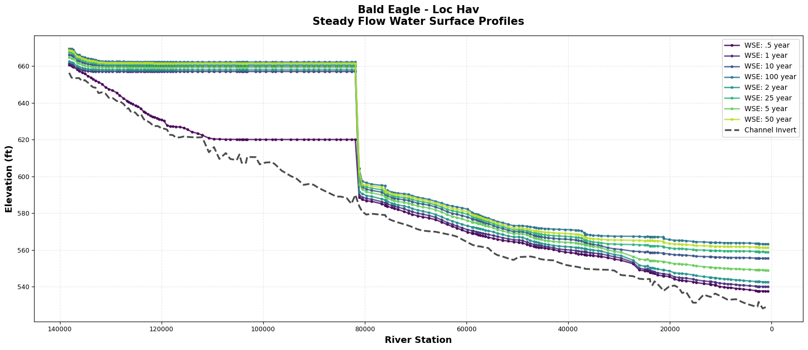
✓ Plotted 8 profiles for Bald Eagle - Loc Hav
  Station range: 659.9 to 138154.4
# Export
Path("working").mkdir(exist_ok=True)
df_steady.to_csv("working/steady_plan02.csv", index=False)
print(f"Exported {len(df_steady)} rows to working/steady_plan02.csv")
Exported 1424 rows to working/steady_plan02.csv
Part 2: Unsteady Time Series (Plan 01)
Extract unsteady results. Note: Methods automatically set Plan 01 as current!
# Run Plan 01 (auto-sets as current, waits for completion)
# This may take 5-10 minutes!
print("Running Plan 01 (Unsteady)...")
# NOTE: Using RasCmdr.compute_plan() instead of RasControl.run_plan()
# because RasControl.run_plan() always sets cores to max
RasCmdr.compute_plan("01", clear_geompre=True, num_cores=2)
print("✓ Plan 01 completed")
2026-07-07 18:15:29 - ras_commander.geom.GeomPreprocessor - INFO - Clearing geometry preprocessor file for single plan: BaldEagle.p01


2026-07-07 18:15:29 - ras_commander.RasCmdr - INFO - Cleared geometry preprocessor files for plan: 01


2026-07-07 18:15:29 - ras_commander.RasUtils - INFO - Successfully updated file: BaldEagle.p01


2026-07-07 18:15:29 - ras_commander.RasCmdr - INFO - Set number of cores to 2 for plan: 01


2026-07-07 18:15:29 - ras_commander.RasCmdr - INFO - Running Ras.exe with -c command line flag for plan 01


Running Plan 01 (Unsteady)...


2026-07-07 18:17:02 - ras_commander.RasCmdr - INFO - HEC-RAS execution completed for plan 01 in 92.75 seconds


✓ Plan 01 completed
# Get output times (auto-sets Plan 01 as current)
times = RasControl.get_output_times("01")
print(f"Found {len(times)} timesteps")
print(f"First: {times[0]}")
print(f"Last: {times[-1]}")
Found 76 timesteps
First: Max WS
Last: 24FEB1999 0400
Extracting Computation Messages (Unsteady Flow)
Similarly, we can extract computation messages for the unsteady flow plan to review: - Simulation timing and performance - Convergence information - Any warnings or errors encountered during computation
# Extract computation messages for unsteady flow Plan 01
print("="*80)
print("COMPUTATION MESSAGES - Plan 01 (Unsteady Flow)")
print("="*80)

msgs_unsteady = RasControl.get_comp_msgs("01")

if msgs_unsteady:
    print(f"\nExtracted {len(msgs_unsteady)} characters of computation messages\n")

    # Display first 800 characters
    print("Computation messages (first 800 characters):")
    print("-" * 80)
    print(msgs_unsteady[:800])

    if len(msgs_unsteady) > 800:
        print("\n... (truncated) ...")

    # Check for errors/warnings
    print("\n" + "="*80)
    print("Checking for warnings/errors...")
    print("="*80)

    lines = msgs_unsteady.split('\n')
    issues = [l for l in lines if 'error' in l.lower() or 'warning' in l.lower()]

    if issues:
        print(f"Found {len(issues)} warning/error lines:")
        for issue in issues[:5]:  # Show first 5
            print(f"  - {issue.strip()}")
    else:
        print("✓ No warnings or errors found")
else:
    print("No computation messages available for Plan 01")

print("\n" + "="*80)
================================================================================
COMPUTATION MESSAGES - Plan 01 (Unsteady Flow)
================================================================================

Extracted 1175 characters of computation messages

Computation messages (first 800 characters):
--------------------------------------------------------------------------------
User selected to use previously computed internal boundary data
but the geometry preprocessor file was for the previous version.
All internal boundary data will be recomputed.

Simulation started at: 14Nov2012 01:29 PM

Writing geometry to output file
Completed writing geometry to output file


Writing plan information to output file
Completed writing plan information to output file


Geometric Preprocessor Version 4.2.0 Jan 2010 XXX XXXX

Finished Processing Geometry
GeomPreprocessor complete - Accepting the preprocessor files.

Performing Unsteady Flow Simulation  Version 4.2.0 Jan 2010 XXX XXXX

Maximum iterations of 20 at:        RS  WSEL    ERROR
20FEB1999 12:44:00  Bald Eagle          Loc Hav             75917.82      592.36       0.012


Finished Unsteady Flow Simulation

Writing Results to DSS
Finishe

... (truncated) ...

================================================================================
Checking for warnings/errors...
================================================================================
Found 1 warning/error lines:
  - Maximum iterations of 20 at:        RS  WSEL    ERROR

================================================================================
# Extract unsteady (limit to 10 timesteps for demo)
df_unsteady = RasControl.get_unsteady_results("01")

print(f"Rows: {len(df_unsteady)}")
print(f"Timesteps: {df_unsteady['time_index'].nunique()}")
print(f"XS: {df_unsteady['node_id'].nunique()}")
df_unsteady.head(10)
Rows: 13528
Timesteps: 76
XS: 178
| river | reach | node_id | time_index | time_string | datetime | wsel | min_ch_el | velocity | flow | froude | energy | max_depth | |
|---|---|---|---|---|---|---|---|---|---|---|---|---|---|
| 0 | Bald Eagle | Loc Hav | 138154.4 | 1 | Max WS | NaT | 672.808289 | 656.299988 | 11.812529 | 7.167449 | 0.546461 | 674.472717 | 16.508301 |
| 1 | Bald Eagle | Loc Hav | 138154.4 | 2 | 18FEB1999 0000 | 1999-02-18 00:00:00 | 660.651123 | 656.299988 | 3.564320 | 1.161268 | 0.352355 | 660.827637 | 4.351135 |
| 2 | Bald Eagle | Loc Hav | 138154.4 | 3 | 18FEB1999 0200 | 1999-02-18 02:00:00 | 660.218872 | 656.299988 | 3.614365 | 1.002599 | 0.376157 | 660.407654 | 3.918884 |
| 3 | Bald Eagle | Loc Hav | 138154.4 | 4 | 18FEB1999 0400 | 1999-02-18 04:00:00 | 661.313293 | 656.299988 | 3.882611 | 1.605426 | 0.361649 | 661.511597 | 5.013306 |
| 4 | Bald Eagle | Loc Hav | 138154.4 | 5 | 18FEB1999 0600 | 1999-02-18 06:00:00 | 662.443420 | 656.299988 | 4.350002 | 2.118352 | 0.357496 | 662.681335 | 6.143433 |
| 5 | Bald Eagle | Loc Hav | 138154.4 | 6 | 18FEB1999 0800 | 1999-02-18 08:00:00 | 663.560730 | 656.299988 | 4.943125 | 2.614835 | 0.367609 | 663.861633 | 7.260742 |
| 6 | Bald Eagle | Loc Hav | 138154.4 | 7 | 18FEB1999 1000 | 1999-02-18 10:00:00 | 664.638428 | 656.299988 | 5.587611 | 3.109273 | 0.383870 | 665.019165 | 8.338440 |
| 7 | Bald Eagle | Loc Hav | 138154.4 | 8 | 18FEB1999 1200 | 1999-02-18 12:00:00 | 665.657776 | 656.299988 | 6.254566 | 3.600435 | 0.403054 | 666.132507 | 9.357788 |
| 8 | Bald Eagle | Loc Hav | 138154.4 | 9 | 18FEB1999 1400 | 1999-02-18 14:00:00 | 666.623291 | 656.299988 | 6.915609 | 4.074730 | 0.422223 | 667.202332 | 10.323303 |
| 9 | Bald Eagle | Loc Hav | 138154.4 | 10 | 18FEB1999 1600 | 1999-02-18 16:00:00 | 667.523621 | 656.299988 | 7.587838 | 4.510049 | 0.440113 | 668.219055 | 11.223633 |
Understanding "Max WS" in Unsteady Output
Important: HEC-RAS unsteady results include a special row with time_string="Max WS" (time_index=1). This contains the maximum values that occurred at ANY computational timestep during the entire simulation, not just at output intervals.
Why this matters: - Output intervals (e.g., every 1 hour) may miss the peak flow/WSE - Computational timesteps (e.g., every 30 seconds) capture the true maximum - "Max WS" shows the absolute peak, even if it wasn't saved to an output interval
How to use it: - Include in DataFrame for reference (critical data!) - Filter out when plotting time series (it's not a timestep) - Show as horizontal reference line on plots to indicate peak
The next cell demonstrates this pattern.
# ============================================================================
# UNSTEADY FLOW: Time Series at Multiple Cross Sections
# ============================================================================
# NOTE: This cell shows LEGACY manual datetime parsing for reference.
# For v0.81.0+, see the cell below for automatic datetime usage!
# ============================================================================

import matplotlib.dates as mdates
import numpy as np

# Convert node_id to float
df_unsteady['node_id'] = df_unsteady['node_id'].astype(float)

# Separate Max WS from timeseries data
df_maxws = df_unsteady[df_unsteady['time_string'] == 'Max WS'].copy()
df_timeseries = df_unsteady[df_unsteady['time_string'] != 'Max WS'].copy()

# LEGACY: Parse datetime for timeseries (NOT NEEDED in v0.81.0+ - datetime column auto-included!)
df_timeseries['datetime'] = pd.to_datetime(df_timeseries['time_string'],
                                           format='%d%b%Y %H%M', errors='coerce')

# Select cross sections to plot (every 20th station for manageable plot count)
all_xs = sorted(df_timeseries['node_id'].unique(), reverse=True)  # Upstream to downstream
selected_xs = all_xs[::20]  # Adjust step size as needed (20, 30, etc.)

if len(selected_xs) == 0:
    selected_xs = [all_xs[0]]  # At least plot one

print(f"Creating time series plots for {len(selected_xs)} cross sections:")
print(f"  Stations: {[f'{xs:.1f}' for xs in selected_xs]}\n")

# Create subplots - one per cross section
n_xs = len(selected_xs)
fig, axes = plt.subplots(n_xs, 1, figsize=(16, 4*n_xs))
if n_xs == 1:
    axes = [axes]

for idx, xs in enumerate(selected_xs):
    ax = axes[idx]

    # Get data for this cross section
    xs_data = df_timeseries[df_timeseries['node_id'] == xs].sort_values('datetime')
    maxws_data = df_maxws[df_maxws['node_id'] == xs]

    if len(xs_data) == 0:
        ax.text(0.5, 0.5, f'No data for station {xs:.1f}',
                ha='center', va='center', transform=ax.transAxes)
        continue

    # Plot WSE time series
    ax.plot(xs_data['datetime'], xs_data['wsel'],
            'b-o', linewidth=2, markersize=5, label='WSE (output intervals)',
            alpha=0.8)

    # Get max values
    max_ws_value = maxws_data['wsel'].iloc[0] if len(maxws_data) > 0 else None
    max_output_value = xs_data['wsel'].max()
    max_output_time = xs_data.loc[xs_data['wsel'].idxmax(), 'datetime']

    # Add horizontal line for computational Max WS
    #if max_ws_value:
    #    ax.axhline(max_ws_value, color='r', linestyle='--',
    #               linewidth=2, alpha=0.7, label='Max WS (computational)')

    # Create annotation text box
    annotation_lines = [
        f"Max WS (computational): {max_ws_value:.2f} ft" if max_ws_value else "Max WS: N/A",
        f"Max (output interval): {max_output_value:.2f} ft",
        f"  at {max_output_time.strftime('%m/%d %H:%M')}" if pd.notna(max_output_time) else ""
    ]
    annotation_text = '\n'.join(annotation_lines)

    ax.text(0.02, 0.98, annotation_text,
            transform=ax.transAxes, fontsize=10,
            verticalalignment='top', horizontalalignment='left',
            bbox=dict(boxstyle='round', facecolor='wheat', alpha=0.9, pad=0.5))

    # Formatting
    ax.set_ylabel('WSE (ft)', fontsize=11, fontweight='bold')
    ax.set_title(f'Station {xs:.1f}', fontsize=12, fontweight='bold', loc='left')
    ax.legend(loc='upper right', fontsize=9, framealpha=0.9)
    ax.grid(True, alpha=0.3, linestyle='--')

    # Format x-axis for dates
    ax.xaxis.set_major_formatter(mdates.DateFormatter('%m/%d\n%H:%M'))
    ax.xaxis.set_major_locator(mdates.HourLocator(interval=6))  # Adjust interval as needed
    plt.setp(ax.xaxis.get_majorticklabels(), rotation=0, ha='center', fontsize=9)

# Add common x-label to bottom subplot
axes[-1].set_xlabel('Date / Time', fontsize=13, fontweight='bold')

plt.suptitle('Unsteady Flow: Water Surface Time Series at Selected Cross Sections',
             fontsize=16, fontweight='bold', y=1.0)
plt.tight_layout()
plt.show()

print(f"\n✓ Created time series plots for {len(selected_xs)} stations")
Creating time series plots for 9 cross sections:
  Stations: ['138154.4', '126454.1', '116401.3', '98206.9', '76643.4', '58836.2', '45233.9', '27226.4', '11865.8']
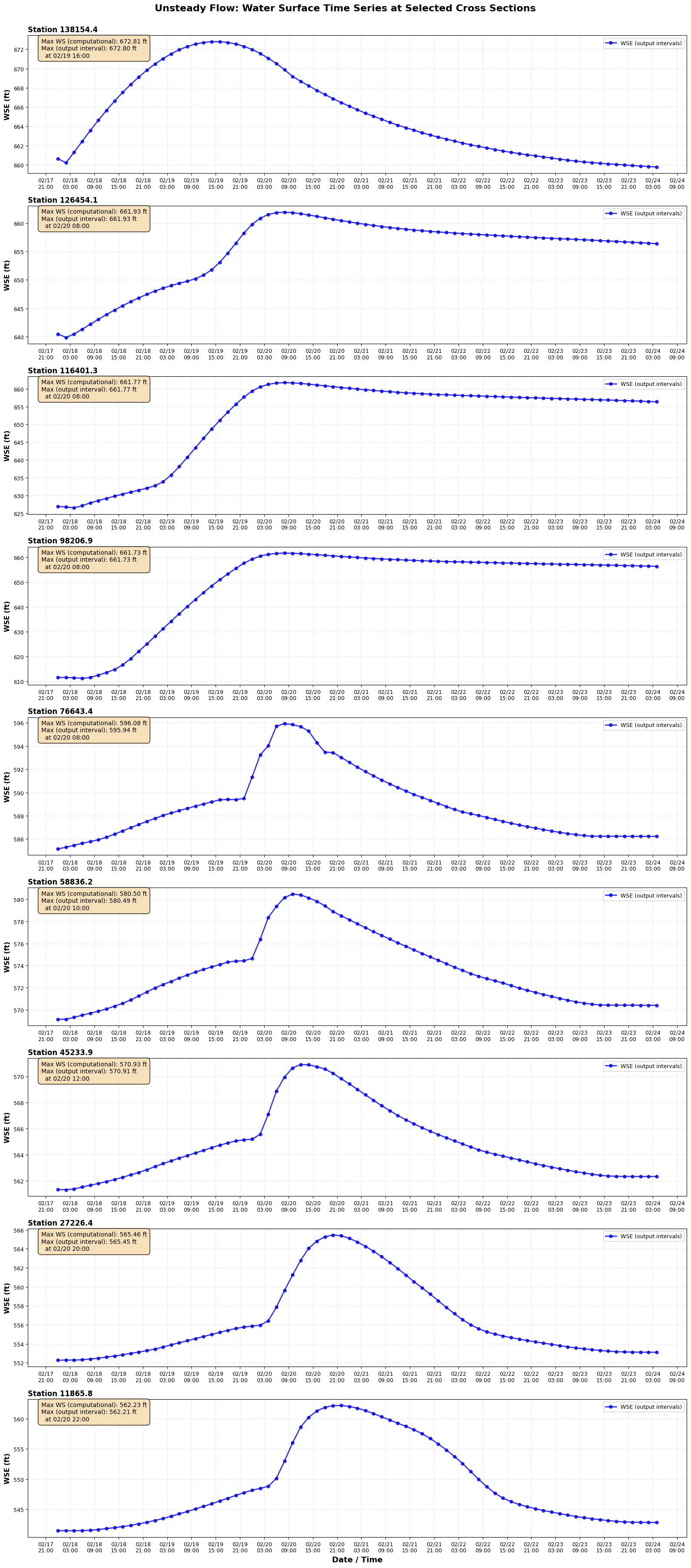
✓ Created time series plots for 9 stations
NEW in v0.81.0: Automatic Datetime Parsing
Starting in version 0.81.0, get_unsteady_results() automatically includes a datetime column with proper datetime64[ns] objects. Manual parsing is no longer needed!
Key Improvements:
- ✅ datetime column added automatically
- ✅ Already in datetime64[ns] format (not strings)
- ✅ "Max WS" rows have pd.NaT for clean filtering
- ✅ Immediate compatibility with pandas datetime operations
- ✅ Backward compatible - time_string still included
The cell above shows the old manual parsing method (kept for reference). The next cell demonstrates the modern approach using the automatic datetime column.
# ============================================================================
# MODERN APPROACH: Using Automatic datetime Column (v0.81.0+)
# ============================================================================

# Check that datetime column exists and is already parsed
print("DataFrame columns:")
print(df_unsteady.columns.tolist())
print(f"\ndatetime column type: {df_unsteady['datetime'].dtype}")
print(f"Sample datetime values:")
print(df_unsteady[['time_string', 'datetime']].head(10))

# Separate using datetime column (NaT for Max WS rows)
df_maxws_modern = df_unsteady[df_unsteady['datetime'].isna()].copy()
df_timeseries_modern = df_unsteady[df_unsteady['datetime'].notna()].copy()

print(f"\nMax WS rows: {len(df_maxws_modern)}")
print(f"Timeseries rows: {len(df_timeseries_modern)}")

# Use pandas datetime accessors directly - no manual parsing needed!
print("\nDatetime operations (no parsing required!):")
print(f"  Simulation start: {df_timeseries_modern['datetime'].min()}")
print(f"  Simulation end: {df_timeseries_modern['datetime'].max()}")
print(f"  Duration: {df_timeseries_modern['datetime'].max() - df_timeseries_modern['datetime'].min()}")
print(f"  Unique hours: {df_timeseries_modern['datetime'].dt.hour.unique()[:10]}")

# Time-based filtering (modern approach)
# Example: Get data for a specific date
specific_date = pd.Timestamp('1999-02-19')
feb_19_data = df_timeseries_modern[df_timeseries_modern['datetime'].dt.date == specific_date.date()]
print(f"\nData points on {specific_date.date()}: {len(feb_19_data)}")

# Example: Get data for specific time range
start_time = pd.Timestamp('1999-02-18 12:00:00')
end_time = pd.Timestamp('1999-02-20 12:00:00')
time_range_data = df_timeseries_modern[
    (df_timeseries_modern['datetime'] >= start_time) &
    (df_timeseries_modern['datetime'] <= end_time)
]
print(f"Data points between {start_time} and {end_time}: {len(time_range_data)}")

print("\n✓ Modern datetime functionality demonstrated")
DataFrame columns:
['river', 'reach', 'node_id', 'time_index', 'time_string', 'datetime', 'wsel', 'min_ch_el', 'velocity', 'flow', 'froude', 'energy', 'max_depth']

datetime column type: datetime64[us]
Sample datetime values:
      time_string            datetime
0          Max WS                 NaT
1  18FEB1999 0000 1999-02-18 00:00:00
2  18FEB1999 0200 1999-02-18 02:00:00
3  18FEB1999 0400 1999-02-18 04:00:00
4  18FEB1999 0600 1999-02-18 06:00:00
5  18FEB1999 0800 1999-02-18 08:00:00
6  18FEB1999 1000 1999-02-18 10:00:00
7  18FEB1999 1200 1999-02-18 12:00:00
8  18FEB1999 1400 1999-02-18 14:00:00
9  18FEB1999 1600 1999-02-18 16:00:00

Max WS rows: 178
Timeseries rows: 13350

Datetime operations (no parsing required!):
  Simulation start: 1999-02-18 00:00:00
  Simulation end: 1999-02-24 04:00:00
  Duration: 6 days 04:00:00
  Unique hours: [ 0  2  4  6  8 10 12 14 16 18]

Data points on 1999-02-19: 2136
Data points between 1999-02-18 12:00:00 and 1999-02-20 12:00:00: 4450

✓ Modern datetime functionality demonstrated
# ============================================================================
# UNSTEADY FLOW: Maximum Water Surface Envelope
# ============================================================================

# Sort by station for profile view
max_wse_sorted = df_maxws.sort_values('node_id', ascending=False)

fig, ax = plt.subplots(figsize=(16, 7))

# Plot maximum WSE envelope
ax.plot(max_wse_sorted['node_id'], max_wse_sorted['wsel'],
        'r-o', linewidth=2.5, markersize=5,
        label='Max WS Envelope (peak at any computational timestep)',
        alpha=0.8)

# Add channel invert
invert = max_wse_sorted[['node_id', 'min_ch_el']].drop_duplicates('node_id').sort_values('node_id', ascending=False)
ax.plot(invert['node_id'], invert['min_ch_el'],
        'k--', linewidth=2.5, alpha=0.7, label='Channel Invert')

# Fill between for visual clarity
ax.fill_between(max_wse_sorted['node_id'],
                max_wse_sorted['min_ch_el'],
                max_wse_sorted['wsel'],
                alpha=0.2, color='blue', label='Maximum Flow Depth')

# Formatting
ax.set_xlabel('River Station', fontsize=13, fontweight='bold')
ax.set_ylabel('Elevation (ft)', fontsize=13, fontweight='bold')
ax.set_title('Maximum Water Surface Envelope\n(Peak elevation reached at any computational timestep during simulation)',
             fontsize=15, fontweight='bold', pad=15)
ax.legend(fontsize=11, loc='best', framealpha=0.9)
ax.grid(True, alpha=0.3, linestyle='--')
ax.invert_xaxis()  # Upstream on left

plt.tight_layout()
plt.show()

# Print summary statistics
max_depth = (max_wse_sorted['wsel'] - max_wse_sorted['min_ch_el']).max()
max_depth_station = max_wse_sorted.loc[(max_wse_sorted['wsel'] - max_wse_sorted['min_ch_el']).idxmax(), 'node_id']

print(f"\n✓ Maximum Water Surface Envelope")
print(f"  Max depth: {max_depth:.2f} ft at station {max_depth_station:.1f}")
print(f"  Highest WSE: {max_wse_sorted['wsel'].max():.2f} ft at station {max_wse_sorted.loc[max_wse_sorted['wsel'].idxmax(), 'node_id']:.1f}")
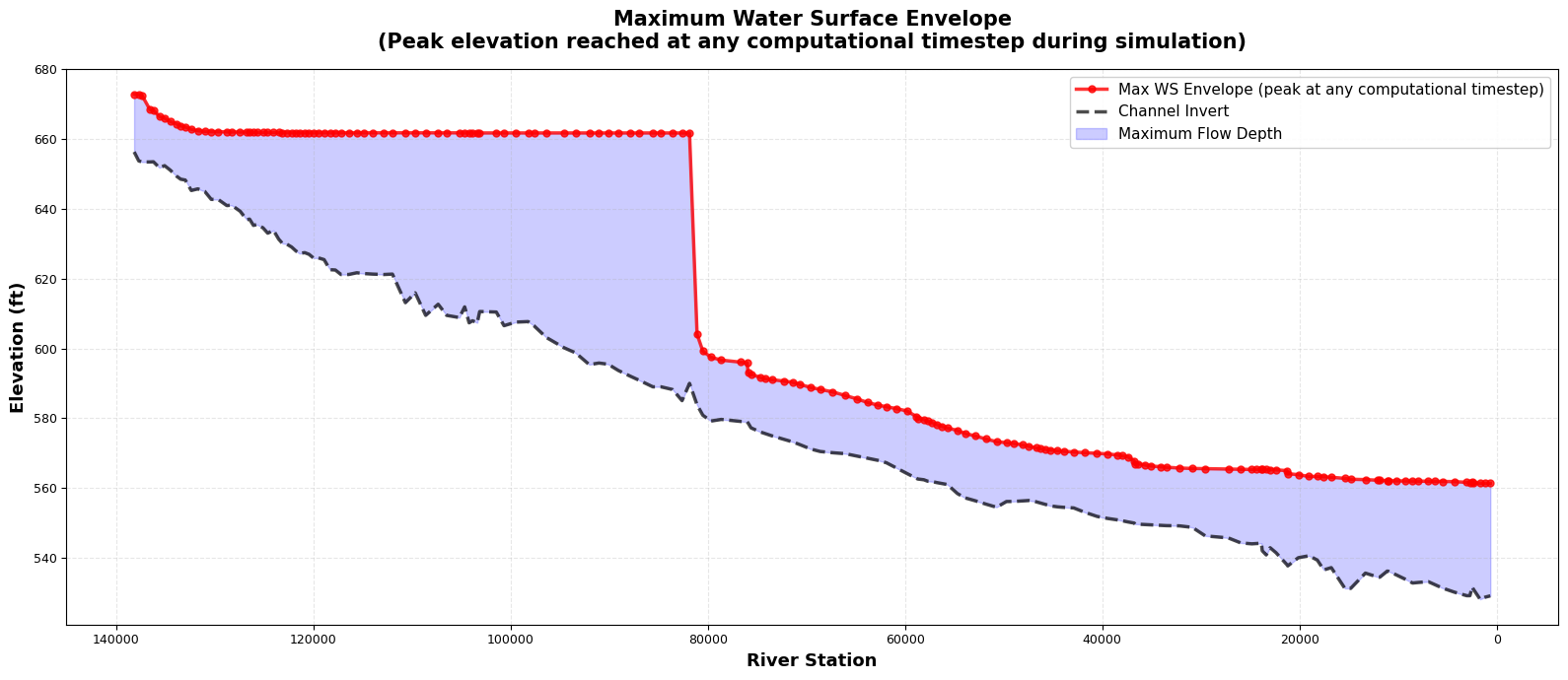
✓ Maximum Water Surface Envelope
  Max depth: 76.66 ft at station 82607.9
  Highest WSE: 672.81 ft at station 138154.4
# ============================================================================
# UNSTEADY FLOW: Velocity Hydrographs at Key Locations
# ============================================================================

# Select critical stations (upstream, middle, downstream)
all_stations = sorted(df_timeseries['node_id'].unique(), reverse=True)
n_stations = len(all_stations)

if n_stations >= 3:
    critical_xs = [
        all_stations[0],                    # Upstream
        all_stations[n_stations // 2],      # Middle
        all_stations[-1]                    # Downstream
    ]
    labels = ['Upstream', 'Midstream', 'Downstream']
else:
    critical_xs = all_stations
    labels = [f'Station {i+1}' for i in range(len(critical_xs))]

fig, ax = plt.subplots(figsize=(14, 6))

colors = ['#1f77b4', '#ff7f0e', '#2ca02c']

# Plot velocity hydrographs
for idx, (xs, label) in enumerate(zip(critical_xs, labels)):
    xs_data = df_timeseries[df_timeseries['node_id'] == xs].sort_values('datetime')
    ax.plot(xs_data['datetime'], xs_data['velocity'],
            marker='o', linewidth=2, markersize=5,
            color=colors[idx % len(colors)],
            label=f'{label} (Sta {xs:.1f})', alpha=0.8)

ax.set_xlabel('Date / Time', fontsize=13, fontweight='bold')
ax.set_ylabel('Velocity (ft/s)', fontsize=13, fontweight='bold')
ax.set_title('Velocity Hydrographs at Key Cross Sections',
              fontsize=14, fontweight='bold')
ax.legend(fontsize=11, loc='best', framealpha=0.9)
ax.grid(True, alpha=0.3, linestyle='--')
ax.xaxis.set_major_formatter(mdates.DateFormatter('%m/%d\n%H:%M'))

plt.tight_layout()
plt.show()

print(f"\n✓ Created velocity hydrographs for {len(critical_xs)} key locations")
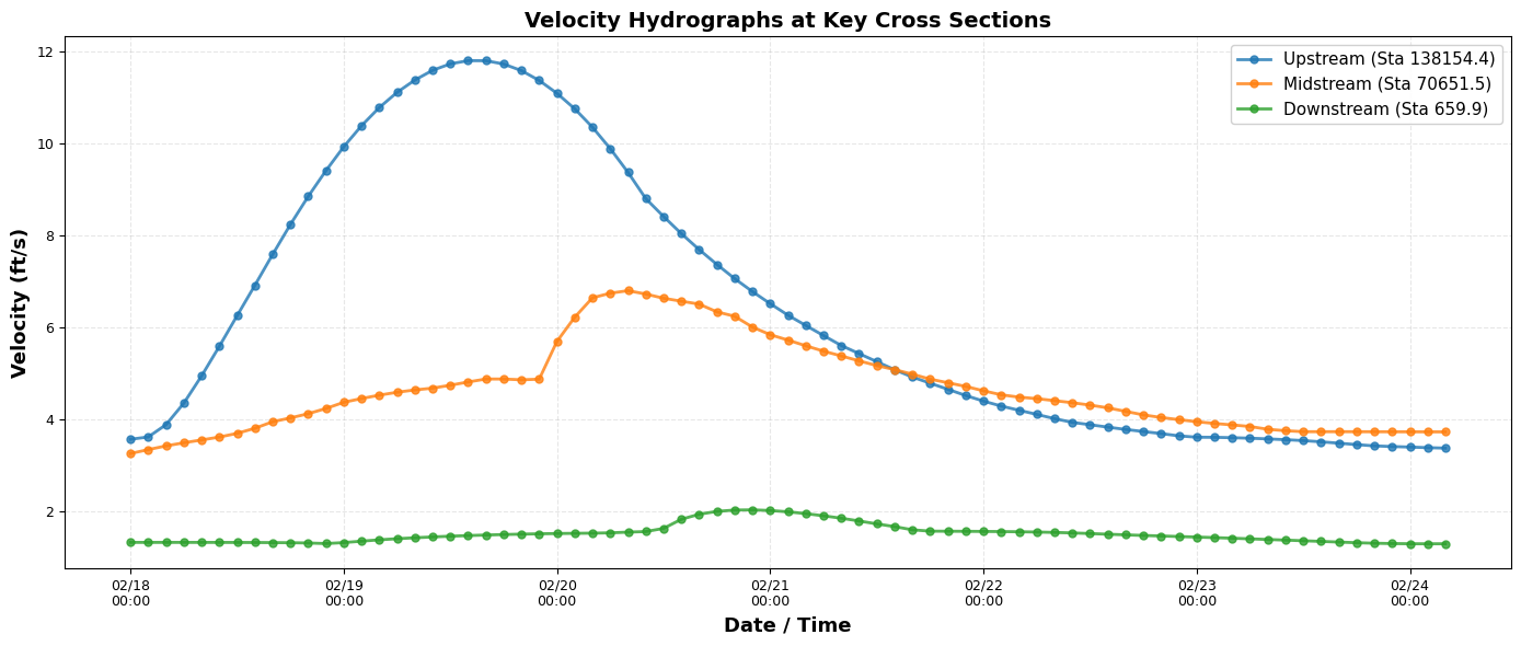
✓ Created velocity hydrographs for 3 key locations
Summary
Complete RasControl API
# Initialize with version (flexible formats)
init_ras_project(path, "4.1")  # or "41", "66", "5.0.6", "506", etc.

# Run plans (auto-sets as current, waits for completion)
# NOTE: run_plan() now checks if plan is current before running
# If results are up-to-date, it skips computation (faster workflow)
success, msgs = RasControl.run_plan("02")

# To force recomputation regardless of current status:
success, msgs = RasControl.run_plan("02", force_recompute=True)

# Extract steady (auto-sets as current)
df_steady = RasControl.get_steady_results("02")

# Extract unsteady (auto-sets as current, includes Max WS)
df_unsteady = RasControl.get_unsteady_results("01")

# Filter for time series plotting
df_timeseries = df_unsteady[df_unsteady['time_string'] != 'Max WS']
max_wse = df_unsteady[df_unsteady['time_string'] == 'Max WS']['wsel'].iloc[0]
Key Features
- ✅ Plan numbers (not file paths)
- ✅ Auto-sets current plan
- ✅ Blocks until completion
- ✅ Steady AND unsteady
- ✅ All versions 3.0-6.7
- ✅ Flexible version formats
- ✅ Includes Max WS data
- ✅ Multi-version comparison (optional)
What Was Demonstrated
- Steady workflow - Plan 02 extraction and plotting
- Unsteady workflow - Plan 01 time series with Max WS reference
- Max WS handling - Understanding and visualizing peak values
- Multi-version comparison - Optional cells for version validation
Next Steps
- Apply to your legacy HEC-RAS models
- Run multi-version comparison for migration validation
- For HEC-RAS 6.0+: Use HDF methods for better performance
19_steady_flow_analysis.ipynb10_1d_hdf_data_extraction.ipynb
What This Creates
Running the multi-version comparison cells will:
New Plans in Project:
- 02_41, 02_506, 02_63, 02_66 (steady)
- 01_41, 01_506, 01_63, 01_66 (unsteady)
CSV Files in working/:
- steady_v41.csv, steady_v506.csv, steady_v63.csv, steady_v66.csv
- unsteady_v41.csv, unsteady_v506.csv, unsteady_v63.csv, unsteady_v66.csv
Results: - All plans remain in project for further analysis - CSV files for external comparison - Plots showing version differences
# =============================================================================
# OPTIONAL: Multi-version unsteady comparison (SKIP for automated testing)
# =============================================================================
# This cell runs multiple HEC-RAS versions and takes 1-2 hours.
# Set SKIP_MULTIVERSION = True to run the comparison.
# =============================================================================

SKIP_MULTIVERSION = True  # Set to False to run optional multi-version comparisons

if SKIP_MULTIVERSION:
    print("Skipping multi-version unsteady comparison (SKIP_MULTIVERSION=True)")
    print("Set SKIP_MULTIVERSION = True in the cell above to run this analysis")
    unsteady_results = {}
    max_ws_data = {}
else:
    from ras_commander import RasPlan

    # Step 1: Update Plan 01 output intervals for more detail
    print("Step 1: Updating Plan 01 intervals...")
    init_ras_project(project_path, RAS_VERSION)  # Use latest for modification

    # Update intervals: Output=15MIN, Mapping=15MIN
    RasPlan.update_plan_intervals("01",
                                  output_interval="10MIN",
                                  mapping_interval="10MIN")
    print("  Output Interval: 1HOUR -> 6MIN")
    print("  Mapping Interval: 1HOUR -> 6MIN\n")

    # Step 2: Run across versions
    # All versions with actual COM interfaces
    test_versions = [
        ("4.1", "41"),       # HEC-RAS 4.1     -> RAS41.HECRASController
    #    ("5.0.1", "501"),    # HEC-RAS 5.0.1   -> RAS501.HECRASController  >> FREEZES, SKIP, LIKELY ISSUE WITH HECRASCONTROLLER
    #    ("5.0.3", "503"),    # HEC-RAS 5.0.3   -> RAS503.HECRASController
        ("5.0.4", "504"),    # HEC-RAS 5.0.4   -> RAS504.HECRASController
        ("5.0.6", "506"),    # HEC-RAS 5.0.6   -> RAS506.HECRASController
        ("6.3.1", "631"),    # HEC-RAS 6.3.1   -> RAS631.HECRASController
        ("6.6", "66"),       # HEC-RAS 6.6     -> RAS66.HECRASController
    ]

    unsteady_results = {}
    max_ws_data = {}  # Store Max WS separately

    print("=== MULTI-VERSION UNSTEADY COMPARISON ===\n")

    for version_name, version_code in test_versions:
        print(f"Processing HEC-RAS {version_name}...")

        # Clone Plan 01 for this version
        new_plan = RasPlan.clone_plan("01",
                          new_shortid=f"Unsteady_{version_code}",
                          new_title=f"Unsteady - v{version_name}")
        print(f"  Cloned to Plan {new_plan}")

        # Re-initialize with this version
        init_ras_project(project_path, version_name)

        # Run the plan (this will take several minutes!)
        print(f"  Running Plan {new_plan} (may take 5-10 min)...")
        # NOTE: Using force_recompute=True for fresh cloned plans to ensure computation
        # (Default behavior now checks if plan is current and skips if already computed)
        #success, msgs = RasControl.run_plan(new_plan, force_recompute=True)
        success, msgs = RasControl.run_plan(new_plan, force_recompute=True)
        print(success, msgs)
        if success:
            # Extract results (limit to 20 timesteps for comparison)
            df = RasControl.get_unsteady_results(new_plan)

            # Separate Max WS from timeseries
            max_ws_data[version_name] = df[df['time_string'] == 'Max WS'].copy()
            unsteady_results[version_name] = df[df['time_string'] != 'Max WS'].copy()

            # Save CSV
            csv_path = Path(f"working/unsteady_v{version_code}.csv")
            df.to_csv(csv_path, index=False)
            print(f"  Extracted {len(df)} rows -> {csv_path}")
        else:
            print(f"  Failed")

        print()
Skipping multi-version unsteady comparison (SKIP_MULTIVERSION=True)
Set SKIP_MULTIVERSION = True in the cell above to run this analysis
# =============================================================================
# Plot multi-version unsteady comparison (if data available)
# =============================================================================

if unsteady_results:
    # Gather all station IDs across versions
    xs_set = set()
    for df in unsteady_results.values():
        try:
            xs_set.update(df['node_id'].astype(float).unique().tolist())
        except Exception:
            xs_set.update(df['node_id'].unique().tolist())

    all_xs = sorted(xs_set, reverse=True)  # upstream -> downstream
    if not all_xs:
        print("No cross section data found in unsteady_results")
    else:
        # Select every 5th cross section for plotting (adjust step as needed)
        step = 5
        selected_xs = all_xs[::step] if len(all_xs) > step else all_xs
        print(f"Plotting {len(selected_xs)} stations (every {step}th of {len(all_xs)} total)")

        for xs_id in selected_xs:
            fig, (ax1, ax2) = plt.subplots(2, 1, figsize=(14, 6))

            # Plot WSE time series for each version at this station
            for version, df in unsteady_results.items():
                # FIX: Convert node_id to float for comparison
                df_float = df.copy()
                df_float['node_id'] = df_float['node_id'].astype(float)
                xs_data = df_float[df_float['node_id'] == xs_id].sort_values('time_index')
                if len(xs_data):
                    ax1.plot(xs_data['time_index'], xs_data['wsel'],
                             marker='o', label=f'v{version}', alpha=0.8)

            # Add Max WS reference lines (if available) for this station
            for version, df in max_ws_data.items():
                try:
                    df_float = df.copy()
                    df_float['node_id'] = df_float['node_id'].astype(float)
                    max_row = df_float[df_float['node_id'] == xs_id]
                    if len(max_row):
                        max_wse = float(max_row['wsel'].iloc[0])
                        ax1.axhline(max_wse, linestyle='--', alpha=0.5, label=f'MaxWS v{version}')
                except Exception:
                    continue

            ax1.set_xlabel('Time Index', fontsize=11)
            ax1.set_ylabel('Water Surface Elevation (ft)', fontsize=11)
            ax1.set_title(f'WSE Time Series at {xs_id} - Version Comparison',
                          fontsize=13, fontweight='bold')
            ax1.legend(fontsize=8)
            ax1.grid(True, alpha=0.3)

            # Plot Flow time series for each version at this station
            for version, df in unsteady_results.items():
                # FIX: Convert node_id to float for comparison
                df_float = df.copy()
                df_float['node_id'] = df_float['node_id'].astype(float)
                xs_data = df_float[df_float['node_id'] == xs_id].sort_values('time_index')
                if len(xs_data):
                    ax2.plot(xs_data['time_index'], xs_data['flow'],
                             marker='o', label=f'v{version}', alpha=0.8)

            ax2.set_xlabel('Time Index', fontsize=11)
            ax2.set_ylabel('Flow (cfs)', fontsize=11)
            ax2.set_title(f'Flow Time Series at {xs_id} - Version Comparison',
                          fontsize=13, fontweight='bold')
            ax2.legend(fontsize=8)
            ax2.grid(True, alpha=0.3)

            plt.tight_layout()
            plt.show()

            # Basic per-station stats
            print(f"\nStation {xs_id}:")
            for version, df in unsteady_results.items():
                df_float = df.copy()
                df_float['node_id'] = df_float['node_id'].astype(float)
                xs_data = df_float[df_float['node_id'] == xs_id]
                if len(xs_data):
                    print(f"  v{version}: timesteps={len(xs_data)}, max_wse={xs_data['wsel'].max():.2f} ft")
                else:
                    print(f"  v{version}: no data")

        # Summary of Max WS across versions for the first selected station (if any)
        if selected_xs:
            summary_xs = selected_xs[0]
            print(f"\nMax WSE by version at station {summary_xs}:")
            for version, df in max_ws_data.items():
                try:
                    df_float = df.copy()
                    df_float['node_id'] = df_float['node_id'].astype(float)
                    max_row = df_float[df_float['node_id'] == summary_xs]
                    if len(max_row):
                        max_wse = float(max_row['wsel'].iloc[0])
                        print(f"  v{version}: {max_wse:.2f} ft")
                    else:
                        print(f"  v{version}: N/A")
                except Exception:
                    print(f"  v{version}: N/A")

else:
    print("Skipping multi-version unsteady comparison plots (no data)")
    print("Set SKIP_MULTIVERSION = True in cell above to run the analysis")
Skipping multi-version unsteady comparison plots (no data)
Set SKIP_MULTIVERSION = True in cell above to run the analysis
Legacy HEC-RAS Automation Reference
HEC Documentation
- HEC-RAS 5.0 User's Manual: Includes COM interface documentation https://www.hec.usace.army.mil/software/hec-ras/documentation.aspx
- Controller Interface Guide: Documentation for HECRASController COM object
COM Interface Limitations
Performance: - Slower than direct file access - Opens GUI (requires active desktop) - Single-threaded (no parallel execution)
Stability: - Depends on HEC-RAS installation - Version-specific (COM interface changes between versions) - Can leave HEC-RAS processes orphaned
Functionality: - Limited to operations HEC-RAS exposes via COM - Cannot access some file-level details - No access to HDF structure (HEC-RAS 5.x)
Modern Alternatives
| Task | Legacy (RasControl) | Modern (HEC-RAS 6.x+) |
|---|---|---|
| Execute plan | RasControl.compute_plan() |
RasCmdr.compute_plan() |
| Extract WSE | RasControl.get_steady_results() |
HdfResultsPlan.get_wse() |
| Extract velocity | RasControl.get_unsteady_results() |
HdfResultsPlan.get_velocity() |
| Modify geometry | COM methods | GeomCrossSection / GeomLateral file parsing |
| Modify plans | COM methods | RasPlan file editing |
Version Comparison Workflow
This notebook demonstrates running same project in multiple HEC-RAS versions for validation:
# Run in HEC-RAS 5.0.7
ras507_results = run_with_version("5.0.7", project_path, "01")

# Run in HEC-RAS 6.3
ras63_results = run_with_version("6.3", project_path, "01")

# Compare results
comparison = compare_wse_profiles(ras507_results, ras63_results)

# Document differences
comparison.to_csv('version_comparison.csv')
Use cases: - Model validation: Confirm results consistent across versions - Migration testing: Verify HEC-RAS upgrade doesn't change results - Regression testing: Detect unexpected changes from HEC-RAS updates
LLM Forward: Multi-Version Documentation
Document version comparison for peer review:
def document_version_comparison(versions_tested, results_dict, output_file):
    import pandas as pd
    import json

    comparison_report = {
        'versions_tested': versions_tested,
        'comparison_date': datetime.now().isoformat(),
        'summary_statistics': {}
    }

    for version, results_df in results_dict.items():
        comparison_report['summary_statistics'][version] = {
            'num_nodes': len(results_df),
            'mean_wse': float(results_df['wse'].mean()),
            'max_wse': float(results_df['wse'].max()),
            'min_wse': float(results_df['wse'].min())
        }

    # Export comparison
    with open(output_file, 'w') as f:
        json.dump(comparison_report, f, indent=2)

    # Also export detailed CSV
    csv_file = output_file.with_suffix('.csv')
    combined_df = pd.concat([
        results_df.assign(version=version)
        for version, results_df in results_dict.items()
    ])
    combined_df.to_csv(csv_file, index=False)

    print(f"Version comparison documented: {output_file}")

# Usage - save to project folder
document_version_comparison(
    versions_tested=["5.0.7", "6.3"],
    results_dict={'5.0.7': ras507_df, '6.3': ras63_df},
    output_file=project_path / 'version_comparison.json'
)
This enables: - Validation documentation: Proof that upgrade doesn't change results - Peer review: Non-programmers can review statistics - Audit trail: Record which versions were compared when
# =============================================================================
# OPTIONAL: Multi-version steady state comparison (SKIP for automated testing)
# =============================================================================
# This cell runs multiple HEC-RAS versions and can take 30+ minutes.
# Set SKIP_MULTIVERSION = True in cell 29 to run this comparison.
# =============================================================================

if SKIP_MULTIVERSION:
    print("Skipping multi-version steady comparison (SKIP_MULTIVERSION=True)")
    print("Set SKIP_MULTIVERSION = True in cell above to run this analysis")
    steady_results = {}
else:
    from ras_commander import RasPlan

    # Versions to test - all versions with actual COM interfaces
    test_versions = [
      #  ("4.1", "41"),       # HEC-RAS 4.1     -> RAS41.HECRASController
      #  ("5.0.1", "501"),    # HEC-RAS 5.0.1   -> RAS501.HECRASController
      #  ("5.0.3", "503"),    # HEC-RAS 5.0.3   -> RAS503.HECRASController
        ("5.0.4", "504"),    # HEC-RAS 5.0.4   -> RAS504.HECRASController
        ("5.0.6", "506"),    # HEC-RAS 5.0.6   -> RAS506.HECRASController
        ("6.3.1", "631"),    # HEC-RAS 6.3.1   -> RAS631.HECRASController
        ("6.6", "66"),       # HEC-RAS 6.6     -> RAS66.HECRASController
    ]

    steady_results = {}

    print("=== MULTI-VERSION STEADY STATE COMPARISON ===\n")

    for version_name, version_code in test_versions:
        print(f"Processing HEC-RAS {version_name}...")

        # Clone Plan 02 for this version
        new_plan = RasPlan.clone_plan("02",
                          new_shortid=f"Steady_{version_code}",
                          new_title=f"Steady - v{version_name}")
        print(f"  Cloned to Plan {new_plan}")

        # Re-initialize with this version
        init_ras_project(project_path, version_name)

        # Run the plan using ras-commander's compute_plan() instead of RasControl.run_plan
        print(f"  Running Plan {new_plan} with 2 cores...")
        try:
            # Use direct command line execution, preferred over RasControl.run_plan
            #RasCmdr.compute_plan(new_plan, clear_geompre=True, num_cores=2)
            success, msgs = RasControl.run_plan(new_plan, force_recompute=True)
            print(success, msgs)
            # Extract results
            df = RasControl.get_steady_results(new_plan)
            steady_results[version_name] = df

            # Save CSV
            csv_path = Path(f"working/steady_v{version_code}.csv")
            df.to_csv(csv_path, index=False)
            print(f"  Extracted {len(df)} rows -> {csv_path}")
        except Exception as e:
            print(f"  Failed: {e}")

        print()

    # Plot comparison - first profile from each version
    if steady_results:
        fig, ax = plt.subplots(figsize=(14, 7))

        for version, df in steady_results.items():
            first_prof = df[df['profile'] == df['profile'].iloc[0]]
            ax.plot(range(len(first_prof)), first_prof['wsel'],
                    marker='o', label=f'v{version}', alpha=0.7)

        ax.set_xlabel('Cross Section Index', fontsize=12)
        ax.set_ylabel('Water Surface Elevation (ft)', fontsize=12)
        ax.set_title('Steady State Profile - Multi-Version Comparison', fontsize=14, fontweight='bold')
        ax.legend(fontsize=10)
        ax.grid(True, alpha=0.3)
        plt.tight_layout()
        plt.show()

        print(f"\nCompared {len(steady_results)} versions")

    else:
        print("No steady results to plot")
Skipping multi-version steady comparison (SKIP_MULTIVERSION=True)
Set SKIP_MULTIVERSION = True in cell above to run this analysis