2D Velocity Profile Line Extraction
Extract velocity, depth, and terrain along a user-defined line from a completed
2D plan. HdfResultsQuery.query_polyline_velocity_profile() uses the native
RasMapperLib velocity renderer through pythonnet. It consumes existing results;
it does not author solver-recorded reference features or rerun the simulation.
| Input | Output |
|---|---|
| Completed plan HDF with face velocity, matching geometry/terrain context, line coordinates in model CRS, and one saved time index | DataFrame containing station, x/y, mesh/face identifiers, velocity components/magnitude, depth, and terrain elevation |
| Sampling spacing in project horizontal units | Station-profile samples; closer spacing does not refine the hydraulic mesh |
The example locates a Bald Eagle result folder through
RAS_COMMANDER_BALD_EAGLE_RESULTS or the local fallbacks below. Those results are
not generated here. Native execution requires compatible installed HEC-RAS/
pythonnet components and resolvable model terrain. See native profile API reference for terrain resolution
and adjacent WSE/depth methods, and 2D profile and reference workflows for choosing the output product.
The saved table and figure retain the original run, including missing velocities. This editorial update does not rerun the calculation or establish accuracy across other projects, terrains, rendering modes, or HEC-RAS versions.
import logging
from pathlib import Path
import os

logging.getLogger("numexpr").setLevel(logging.WARNING)
logging.getLogger("numexpr.utils").setLevel(logging.WARNING)

import h5py
import matplotlib.pyplot as plt
from matplotlib.ticker import MaxNLocator, ScalarFormatter
import numpy as np
from shapely.geometry import LineString

from ras_commander import HdfResultsQuery

plt.rcParams.update({
    "figure.dpi": 130,
    "axes.grid": True,
    "grid.alpha": 0.25,
    "axes.spines.top": False,
    "axes.spines.right": False,
})
Locate Completed Bald Eagle Results
def candidate_result_dirs():
    env_path = os.environ.get("RAS_COMMANDER_BALD_EAGLE_RESULTS")
    if env_path:
        yield Path(env_path)
    yield Path("H:/Symphony/RASDecomp/CLB-850/inputs/BaldEagleCrkMulti2D_722_gridded")

    workspace = Path.cwd()
    for root in [workspace, *workspace.parents[:3]]:
        yield root / "example_projects" / "BaldEagleCrkMulti2D_velocity"
        yield root / "examples" / "example_projects" / "BaldEagleCrkMulti2D_AORC_2020_901"


def find_plan_hdf():
    for result_dir in candidate_result_dirs():
        if not result_dir.exists():
            continue
        for plan_hdf in sorted(result_dir.glob("BaldEagleDamBrk.p*.hdf")):
            with h5py.File(plan_hdf, "r") as hdf:
                if "Geometry/2D Flow Areas/Attributes" not in hdf:
                    continue
                mesh_name = hdf["Geometry/2D Flow Areas/Attributes"][()]["Name"][0].decode().strip()
                face_velocity_path = (
                    "Results/Unsteady/Output/Output Blocks/Base Output/"
                    f"Unsteady Time Series/2D Flow Areas/{mesh_name}/Face Velocity"
                )
                if face_velocity_path in hdf:
                    return plan_hdf, mesh_name
    raise FileNotFoundError(
        "Completed Bald Eagle result HDF not found. Set "
        "RAS_COMMANDER_BALD_EAGLE_RESULTS to a folder containing BaldEagleDamBrk.p##.hdf."
    )


plan_hdf, mesh_name = find_plan_hdf()
print(f"Using {plan_hdf.name} from {plan_hdf.parent.name}; mesh={mesh_name}")
Using BaldEagleDamBrk.p07.hdf from BaldEagle; mesh=BaldEagleCr
Build A Profile Line Through Peak Face Velocity
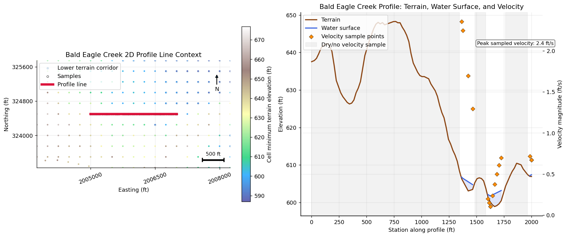
The code identifies the saved time with the largest absolute face velocity in the selected mesh, then draws a horizontal 2,000-model-unit line through an adjacent cell center. This creates an inspection transect, not a channel centerline or an automatically engineered cross section.
time_index identifies one saved output time. It does not mean maximum
velocity at every station; the native velocity API rejects time_index="max".
Compare WSE, depth, and velocity at the same concrete time with compatible terrain
and rendering assumptions. Use the native WSE/depth profile methods in the API
reference rather than treating all HDF arrays as interchangeable surfaces.
The spacing is 100 model units. The renderer may emit additional breakpoints or
repeated stations; inspect the table before resampling. wet_profile below
filters only rows with a mesh assignment: its name does not guarantee positive
depth or finite velocity. Keep missing values visible and distinguish outside-mesh,
dry, and unresolved samples during review.
with h5py.File(plan_hdf, "r") as hdf:
    base_geom = f"Geometry/2D Flow Areas/{mesh_name}"
    face_velocity_path = (
        "Results/Unsteady/Output/Output Blocks/Base Output/"
        f"Unsteady Time Series/2D Flow Areas/{mesh_name}/Face Velocity"
    )
    face_velocity = np.asarray(hdf[face_velocity_path][()])
    time_index = int(np.nanargmax(np.nanmax(np.abs(face_velocity), axis=1)))
    peak_face_id = int(np.nanargmax(np.abs(face_velocity[time_index])))
    face_cells = np.asarray(hdf[f"{base_geom}/Faces Cell Indexes"][peak_face_id])
    seed_cell = int(face_cells[face_cells >= 0][0])
    seed_xy = np.asarray(hdf[f"{base_geom}/Cells Center Coordinate"][seed_cell], dtype=float)

profile_line = LineString([
    (float(seed_xy[0] - 1000.0), float(seed_xy[1])),
    (float(seed_xy[0] + 1000.0), float(seed_xy[1])),
])

profile = HdfResultsQuery.query_polyline_velocity_profile(
    plan_hdf,
    profile_line,
    time_index=time_index,
    sample_spacing=100.0,
)
wet_profile = profile[profile["mesh_name"].notna()].copy()
if wet_profile.empty:
    raise RuntimeError("Profile line did not intersect wet 2D mesh output.")

profile.head()
| station | x | y | mesh_name | face_id | velocity_x | velocity_y | velocity_mag | depth | terrain_elev | |
|---|---|---|---|---|---|---|---|---|---|---|
| 0 | 0.000000 | 2.005100e+06 | 324500.0 | BaldEagleCr | 170460 | NaN | NaN | NaN | NaN | 641.638367 |
| 1 | 0.000000 | 2.005100e+06 | 324500.0 | BaldEagleCr | 170460 | NaN | NaN | NaN | NaN | 641.638367 |
| 2 | 15.670330 | 2.005116e+06 | 324500.0 | BaldEagleCr | 170671 | NaN | NaN | NaN | NaN | 642.000305 |
| 3 | 44.535305 | 2.005145e+06 | 324500.0 | BaldEagleCr | 170671 | NaN | NaN | NaN | NaN | 642.375122 |
| 4 | 50.000000 | 2.005150e+06 | 324500.0 | BaldEagleCr | 170671 | NaN | NaN | NaN | NaN | 642.157410 |
Plot Velocity Against Terrain
The left panel locates the line and samples. The right panel plots returned terrain, terrain-plus-depth, and velocity magnitude versus station. Missing velocities remain gaps rather than becoming zero. Velocity magnitude is speed, not signed transect-normal velocity or integrated discharge.
These Bald Eagle labels assume feet and ft/s. Confirm coordinate units, vertical datum, depth definition, and velocity units when adapting the figure. For batch plots, keep line name, plan, saved time, terrain, sample spacing, returned provenance, and output filename alongside every figure. Retain failed or empty profiles for review instead of silently omitting them.
314 demonstrates a per-line plotting loop for recorded reference results; 413 demonstrates flow-versus-time extraction. Neither establishes that every spatial renderer or variable matches the RASMapper GUI. Such comparisons must match vertices, selected plan/time, terrain association, and rendering method.
with h5py.File(plan_hdf, "r") as hdf:
    base_geom = f"Geometry/2D Flow Areas/{mesh_name}"
    centers = np.asarray(hdf[f"{base_geom}/Cells Center Coordinate"][()], dtype=float)
    cell_min = np.asarray(hdf[f"{base_geom}/Cells Minimum Elevation"][()], dtype=float)

pad = 1250.0
xmin, ymin, xmax, ymax = profile_line.bounds
near_mask = (
    (centers[:, 0] >= xmin - pad)
    & (centers[:, 0] <= xmax + pad)
    & (centers[:, 1] >= ymin - pad)
    & (centers[:, 1] <= ymax + pad)
)

fig, (ax_map, ax_profile) = plt.subplots(
    1,
    2,
    figsize=(14.0, 5.8),
    gridspec_kw={"width_ratios": [1.0, 1.25]},
    constrained_layout=True,
)

low_terrain_threshold = np.nanpercentile(cell_min[near_mask], 20.0)
low_terrain_mask = near_mask & (cell_min <= low_terrain_threshold)
ax_map.scatter(
    centers[low_terrain_mask, 0],
    centers[low_terrain_mask, 1],
    s=18,
    color="steelblue",
    alpha=0.22,
    linewidths=0,
    label="Lower terrain corridor",
)
terrain_scatter = ax_map.scatter(
    centers[near_mask, 0],
    centers[near_mask, 1],
    c=cell_min[near_mask],
    s=8,
    cmap="terrain",
    alpha=0.75,
    linewidths=0,
)
ax_map.scatter(wet_profile["x"], wet_profile["y"], s=12, facecolors="white", edgecolors="black", linewidths=0.6, alpha=0.85, label="Samples", zorder=4)
line_x, line_y = profile_line.xy
ax_map.plot(line_x, line_y, color="crimson", linewidth=4.2, label="Profile line", zorder=6)
ax_map.annotate("N", xy=(0.93, 0.88), xytext=(0.93, 0.73), xycoords="axes fraction", ha="center", va="center", arrowprops={"arrowstyle": "-|>", "lw": 1.4})
ax_map.set_xlim(xmin - pad, xmax + pad)
ax_map.set_ylim(ymin - pad, ymax + pad)
scale_len = 500.0
scale_x0 = xmax + pad - scale_len - 150.0
scale_y0 = ymin - pad + 180.0
ax_map.plot([scale_x0, scale_x0 + scale_len], [scale_y0, scale_y0], color="black", linewidth=3.0, solid_capstyle="butt", zorder=5)
ax_map.plot([scale_x0, scale_x0], [scale_y0 - 35.0, scale_y0 + 35.0], color="black", linewidth=2.0, zorder=5)
ax_map.plot([scale_x0 + scale_len, scale_x0 + scale_len], [scale_y0 - 35.0, scale_y0 + 35.0], color="black", linewidth=2.0, zorder=5)
ax_map.text(scale_x0 + scale_len / 2.0, scale_y0 + 80.0, "500 ft", ha="center", va="bottom", fontsize=9, bbox={"facecolor": "white", "edgecolor": "none", "alpha": 0.85})
ax_map.set_title("Bald Eagle Creek 2D Profile Line Context")
ax_map.set_xlabel("Easting (ft)")
ax_map.set_ylabel("Northing (ft)")
ax_map.set_aspect("equal", adjustable="box")
for axis in (ax_map.xaxis, ax_map.yaxis):
    formatter = ScalarFormatter(useOffset=False)
    formatter.set_scientific(False)
    axis.set_major_formatter(formatter)
    axis.set_major_locator(MaxNLocator(nbins=4))
ax_map.tick_params(axis="x", labelrotation=20)
ax_map.legend(loc="upper left", frameon=True)
cbar = fig.colorbar(terrain_scatter, ax=ax_map, shrink=0.86)
cbar.set_label("Cell minimum terrain elevation (ft)")

station = wet_profile["station"].to_numpy(dtype=float)
terrain = wet_profile["terrain_elev"].to_numpy(dtype=float)
water_surface = terrain + wet_profile["depth"].to_numpy(dtype=float)
velocity_mag = wet_profile["velocity_mag"].to_numpy(dtype=float)
missing_velocity = ~np.isfinite(velocity_mag)
gap_patch = None
if np.any(missing_velocity):
    gap_indexes = np.flatnonzero(missing_velocity)
    gap_groups = np.split(gap_indexes, np.where(np.diff(gap_indexes) > 1)[0] + 1)
    for gap_group in gap_groups:
        if len(gap_group) == 0:
            continue
        start_station = float(station[gap_group[0]])
        end_station = float(station[gap_group[-1]])
        if np.isclose(start_station, end_station):
            end_station = start_station + 20.0
        span = ax_profile.axvspan(start_station, end_station, color="0.82", alpha=0.28, label="Dry/no velocity sample" if gap_patch is None else None)
        if gap_patch is None:
            gap_patch = span
drop_patch = None
if len(station) > 1:
    drop_idx = int(np.nanargmin(np.diff(terrain)))
    drop_station0 = float(station[drop_idx])
    drop_station1 = float(station[drop_idx + 1])
    terrain_drop = float(terrain[drop_idx] - terrain[drop_idx + 1])
    if terrain_drop > 5.0:
        drop_patch = ax_profile.axvspan(drop_station0, drop_station1, color="gold", alpha=0.18, label="Steep terrain drop")

terrain_line, = ax_profile.plot(station, terrain, color="saddlebrown", linewidth=2.0, label="Terrain")
wse_line, = ax_profile.plot(station, water_surface, color="royalblue", linewidth=2.0, label="Water surface")
ax_profile.fill_between(station, terrain, water_surface, color="royalblue", alpha=0.16)
ax_profile.set_title("Bald Eagle Creek Profile: Terrain, Water Surface, and Velocity")
ax_profile.set_xlabel("Station along profile (ft)")
ax_profile.set_ylabel("Elevation (ft)")
if drop_patch is not None:
    ax_profile.annotate(
        f"Steep terrain drop\n{terrain_drop:.0f} ft over {drop_station1 - drop_station0:.0f} ft",
        xy=((drop_station0 + drop_station1) / 2.0, min(terrain[drop_idx], terrain[drop_idx + 1]) + 12.0),
        xytext=(drop_station1 + 130.0, min(terrain[drop_idx], terrain[drop_idx + 1]) + 34.0),
        arrowprops={"arrowstyle": "->", "color": "saddlebrown", "lw": 1.1},
        color="saddlebrown",
        fontsize=9,
        bbox={"boxstyle": "round,pad=0.25", "facecolor": "white", "edgecolor": "saddlebrown", "alpha": 0.9},
    )

ax_velocity = ax_profile.twinx()
velocity_line = ax_velocity.scatter(station, velocity_mag, s=30, marker="D", color="darkorange", edgecolors="black", linewidths=0.35, label="Velocity sample points", zorder=5)
ax_velocity.set_ylabel("Velocity magnitude (ft/s)")
peak_idx = int(np.nanargmax(velocity_mag))
peak_station = float(station[peak_idx])
peak_velocity = float(velocity_mag[peak_idx])
ax_velocity.text(
    0.73,
    0.84,
    f"Peak sampled velocity: {peak_velocity:.1f} ft/s",
    transform=ax_velocity.transAxes,
    color="black",
    fontsize=9,
    bbox={"boxstyle": "round,pad=0.25", "facecolor": "white", "edgecolor": "0.35", "alpha": 0.92},
)

lines = [terrain_line, wse_line, velocity_line]
if drop_patch is not None:
    lines.append(drop_patch)
if gap_patch is not None:
    lines.append(gap_patch)
ax_profile.legend(lines, [line.get_label() for line in lines], loc="upper left", frameon=True)
plt.show()