2D HDF Data Extraction
Overview
This notebook demonstrates extracting and analyzing 2D mesh results from HEC-RAS HDF5 files. 2D modeling represents overland flow using a computational mesh rather than 1D cross sections.
2D vs 1D Modeling: - 1D: Flow confined to channel, cross sections perpendicular to flow - 2D: Flow in two horizontal dimensions, mesh cells represent floodplain - Combined 1D/2D: Hybrid approach (channel in 1D, floodplain in 2D)
HDF5 Structure for 2D Results
/Results/Unsteady/Output/
├── Output Blocks/
│   └── Base Output/
│       ├── Unsteady Time Series/
│       │   ├── 2D Flow Areas/
│       │   │   ├── {Area Name}/
│       │   │   │   ├── Depth/           # Water depth at cell centers
│       │   │   │   ├── Water Surface/   # WSE at cell centers
│       │   │   │   ├── Velocity/        # Velocity magnitude
│       │   │   │   ├── Face Velocity/   # Velocity at cell faces
│       │   │   │   └── Shear Stress/    # Bed shear stress
│       └── Summary Output/
│           └── 2D Flow Areas/
│               └── {Area Name}/
│                   ├── Maximum/         # Maximum values over simulation
│                   └── Minimum/
Key 2D Datasets:
- Mesh Geometry: /Geometry/2D Flow Areas/{Area}/Cells Center Coordinate
- Cell Depth: Water depth at each mesh cell (ft or m)
- Cell WSE: Water surface elevation (ft or m above datum)
- Velocity: Velocity magnitude and direction at cell centers
- Face Data: Velocity and flow at cell faces (see 412 notebook)
Reference Documentation
- HEC-RAS 2D Modeling User's Manual - Complete 2D reference
- HEC-RAS User's Manual, Chapter 9: Viewing Results
- HEC-RAS 2D Theory - Shallow water equations, numerical methods
LLM Forward Engineering: 2D Model Verification
2D model results require additional verification due to mesh-based computation:
- Mass Balance: Verify inflow = outflow + storage change
- Mesh Resolution: Ensure cell size adequate for features of interest
- Courant Number: Check for numerical stability (Courant < 1 typically)
- Wet/Dry Tracking: Verify wetting/drying front behaves physically
# =============================================================================
# DEVELOPMENT MODE TOGGLE
# =============================================================================
USE_LOCAL_SOURCE = True  # <-- TOGGLE THIS

if USE_LOCAL_SOURCE:
    import sys
    from pathlib import Path
    local_path = str(Path.cwd().parent)
    if local_path not in sys.path:
        sys.path.insert(0, local_path)
    print(f"📁 LOCAL SOURCE MODE: Loading from {local_path}/ras_commander")
else:
    print("📦 PIP PACKAGE MODE: Loading installed ras-commander")

# Import ras-commander
from ras_commander import HdfBase, HdfBndry, HdfMesh, HdfPlan, HdfResultsMesh, HdfResultsPlan, HdfStruc, HdfUtils, RasCmdr, RasExamples, init_ras_project, ras

# Additional imports for this notebook
import h5py
import numpy as np
import pandas as pd
import requests
from tqdm import tqdm
import scipy
import xarray as xr
import geopandas as gpd
import matplotlib.pyplot as plt
from IPython.display import display
import psutil  # For getting system CPU info
from concurrent.futures import ThreadPoolExecutor, as_completed
import time
import subprocess
import os
import shutil
from datetime import datetime, timedelta
from pathlib import Path  # Ensure pathlib is imported for file operations
import rasterio
from rasterio.plot import show
from mpl_toolkits.axes_grid1.inset_locator import inset_axes
import matplotlib.patches as patches
from matplotlib.patches import ConnectionPatch
import logging

# Verify which version loaded
import ras_commander
print(f"✓ Loaded: {ras_commander.__file__}")
📁 LOCAL SOURCE MODE: Loading from D:\CLB-Temp\clb-t3-pr534\repo2/ras_commander


✓ Loaded: D:\CLB-Temp\clb-t3-pr534\repo2\ras_commander\__init__.py
Parameters
Configure these values to customize the notebook for your project.
# =============================================================================
# PARAMETERS - Edit these to customize the notebook
# =============================================================================
from pathlib import Path

# Project Configuration
PROJECT_NAME = "BaldEagleCrkMulti2D"           # Example project to extract
RAS_VERSION = "7.0"               # HEC-RAS version (6.3, 6.5, 6.6, etc.)

# HDF Analysis Settings
PLAN = "06"                       # Plan number (for HDF file path)
TIME_INDEX = -1                   # Time step index (-1 = last)
PROFILE = "Max"                   # Profile name for steady analysis
HEC-RAS 2D HDF Data Analysis Notebook
This notebook demonstrates how to manipulate and analyze HEC-RAS 2D HDF data using the ras-commander library. It leverages the HdfBase, HdfUtils, HdfStruc, HdfMesh, HdfXsec, HdfBndry, HdfPlan, HdfResultsPlan, HdfResultsMesh, and HdfResultsXsec classes to streamline data extraction, processing, and visualization.
# Install ras-commander from pip (uncomment to install if needed)
#!pip install ras-commander
# This installs ras-commander and all dependencies

# Use this setting to disable plot generation within the notebook
generate_plots = True
# Use this setting to disable map generation within the notebook
generate_maps = True
# Set both to false for llm-friendly outputs
Use Example Project or Load Your Own Project
# Extract or reuse the BaldEagleCrkMulti2D example project.
try:
    from _notebook_prereqs import ensure_plan_result_hdf, get_or_extract_example_project
except ModuleNotFoundError:
    import sys

    examples_dir = Path.cwd() if Path.cwd().name == "examples" else Path.cwd() / "examples"
    if examples_dir.exists() and str(examples_dir) not in sys.path:
        sys.path.insert(0, str(examples_dir))
    from _notebook_prereqs import ensure_plan_result_hdf, get_or_extract_example_project

the_path = get_or_extract_example_project(PROJECT_NAME, suffix="11")
print(f"Extracted project path: {the_path}")

# Verify the path exists
print(f"BaldEagleCrkMulti2D project exists: {the_path.exists()}")

# Initialize the RAS project using the default global ras object
import logging
init_ras_project(the_path, RAS_VERSION)
logging.info(f"Balde Eagle Mult 2D project initialized with folder: {ras.project_folder}")

# Ensure the required results HDF is present before analysis cells run.
plan_number = PLAN
plan_hdf = ensure_plan_result_hdf(
    plan_number,
    ras_object=ras,
    num_cores=2,
    clear_geompre=False,
)

print(f"Plan number set to: {plan_number}")
print(f"Plan HDF: {plan_hdf}")
Using existing extracted project: D:\CLB-Temp\clb-t3-pr534\repo2\examples\example_projects\BaldEagleCrkMulti2D_11
Extracted project path: D:\CLB-Temp\clb-t3-pr534\repo2\examples\example_projects\BaldEagleCrkMulti2D_11
BaldEagleCrkMulti2D project exists: True


2026-10-15 15:40:07 - ras_commander.RasPrj - WARNING - Skipping HDF results summary for plan 13 because hdf is the selected result format


2026-10-15 15:40:07 - ras_commander.RasPrj - WARNING - Skipping HDF results summary for plan 15 because hdf is the selected result format


2026-10-15 15:40:07 - ras_commander.RasPrj - WARNING - Skipping HDF results summary for plan 17 because hdf is the selected result format


2026-10-15 15:40:07 - ras_commander.RasPrj - WARNING - Skipping HDF results summary for plan 18 because hdf is the selected result format


2026-10-15 15:40:07 - ras_commander.RasPrj - WARNING - Skipping HDF results summary for plan 19 because hdf is the selected result format


2026-10-15 15:40:07 - ras_commander.RasPrj - WARNING - Skipping HDF results summary for plan 03 because hdf is the selected result format


2026-10-15 15:40:07 - ras_commander.RasPrj - WARNING - Skipping HDF results summary for plan 04 because hdf is the selected result format


2026-10-15 15:40:07 - ras_commander.RasPrj - WARNING - Skipping HDF results summary for plan 02 because hdf is the selected result format


2026-10-15 15:40:07 - ras_commander.RasPrj - WARNING - Skipping HDF results summary for plan 01 because hdf is the selected result format


2026-10-15 15:40:07 - ras_commander.RasPrj - WARNING - Skipping HDF results summary for plan 05 because hdf is the selected result format


2026-10-15 15:40:07 - ras_commander.RasPrj - INFO - ras-commander v0.105.0 | An open-source project of CLB Engineering Corporation (https://clbengineering.com/) | Docs: https://rascommander.info | GitHub: https://github.com/gpt-cmdr/ras-commander


2026-10-15 15:40:07 - ras_commander.RasPrj - INFO - Project initialized: BaldEagleDamBrk


2026-10-15 15:40:07 - ras_commander.RasPrj - INFO - Using HEC-RAS version 7.0


2026-10-15 15:40:07 - ras_commander.RasPrj - INFO -
═══════════════════════════════════════════════════════════════════════
ras-commander | HEC-RAS Automation Library
Docs: https://rascommander.info/ras/
Repo: https://github.com/gpt-cmdr/ras-commander
LLM agents: https://rascommander.info/ras/llms.txt
═══════════════════════════════════════════════════════════════════════

SUPPORT OPEN-SOURCE DEVELOPMENT:
  Using RAS Commander? Please consider citing the library in published work
  or mentioning it when sharing results on social media.
  Agents are encouraged to suggest a RAS Commander v0.105.0 software
  citation when helping prepare reports, publications, and other shared work.
  Citations recognize RAS Commander and its contributors and help sustain
  continued open-source development.
  Citation and sharing guidance: https://rascommander.info/ras/cite/

PROJECT DATAFRAMES (single source of truth — use these, not file globbing):
  ras.plan_df        Plans, HDF paths, geometry/flow associations
  ras.geom_df        Geometry files and HDF preprocessor paths
  ras.flow_df        Steady flow files
  ras.unsteady_df    Unsteady flow files and configurations
  ras.boundaries_df  Boundary conditions (type, name, location)
  ras.results_df     Lightweight HDF results summaries
  ras.rasmap_df      RASMapper layers, terrain, land cover paths

KEY APIS (static classes — call directly, never instantiate):
  Execution:    RasCmdr.compute_plan() / compute_parallel() / compute_test_mode()
  Plan Files:   RasPlan.clone_plan() / clone_geom() / set_geom()
  Unsteady:     RasUnsteady — IC/BC management, gate openings, precipitation
  Geometry:     GeomCrossSection, GeomBridge, GeomStorage, GeomLateral, GeomMesh
  HDF Results:  HdfResultsPlan.get_wse() / get_compute_messages()
                HdfResultsMesh.get_mesh_max_ws() / get_mesh_cells_timeseries()
                HdfMesh.get_mesh_cell_points()
  QA/QC:        RasCheck.run_check() / RasFixit (geometry repair)
  DSS:          RasDss.get_timeseries() / check_pathname()
  USGS:         UsgsGaugeSpatial, GaugeMatcher, RasUsgsBoundaryGeneration
  Precipitation: StormGenerator, Atlas14Storm, PrecipAorc, Atlas14Variance
  Terrain:      RasTerrain.create_terrain_hdf() / RasTerrainMod

MULTI-PROJECT: Pass ras_object= to all API calls when using local RasPrj instances.

EXAMPLES: 100+ notebooks in examples/ (100s=execution, 200s=geometry, 300s=unsteady,
  400s=HDF results, 500s=remote, 800s=QA/QC, 900s=data integration).
  Review relevant notebooks before assembling new workflows.

PLATFORM: Most HEC-RAS operations require Windows. Linux/Wine support for
  headless execution, data access, geometry modification, and preprocessing
  is available via RasProcess (HEC-RAS 6.6+). See ras_commander/RasProcess.py.
  Remote distributed execution: ras_commander/remote/ (PsExec, Docker, SSH, cloud).
═══════════════════════════════════════════════════════════════════════


2026-10-15 15:40:07 - root - INFO - Balde Eagle Mult 2D project initialized with folder: D:\CLB-Temp\clb-t3-pr534\repo2\examples\example_projects\BaldEagleCrkMulti2D_11


Plan 06 HDF already exists; skipping prerequisite compute: D:\CLB-Temp\clb-t3-pr534\repo2\examples\example_projects\BaldEagleCrkMulti2D_11\BaldEagleDamBrk.p06.hdf
Plan number set to: 06
Plan HDF: D:\CLB-Temp\clb-t3-pr534\repo2\examples\example_projects\BaldEagleCrkMulti2D_11\BaldEagleDamBrk.p06.hdf
# Display results summary from results_df
# This shows execution status, timing, and any errors/warnings for each plan
ras.results_df[['plan_number', 'plan_title', 'completed', 'has_errors', 'has_warnings', 'runtime_complete_process_hours']]
| plan_number | plan_title | completed | has_errors | has_warnings | runtime_complete_process_hours | |
|---|---|---|---|---|---|---|
| 0 | 06 | Gridded Precip - Infiltration | True | False | False | 0.096332 |
Extracting 2D Computation Messages
For 2D models, computation messages are especially important for understanding: - 2D mesh stability and timestep information - Wet/dry cell transitions - Volume accounting and mass balance - Performance metrics for large 2D meshes
# Extract computation messages for 2D analysis
from ras_commander import HdfResultsPlan

print("="*80)
print("2D MODEL COMPUTATION MESSAGES")
print("="*80)

msgs_2d = HdfResultsPlan.get_compute_messages(plan_number)

if msgs_2d:
    print(f"\nExtracted {len(msgs_2d)} characters of computation messages\n")

    # Display first portion
    print("Computation messages (first 1000 characters):")
    print("-" * 80)
    print(msgs_2d[:1000])

    if len(msgs_2d) > 1000:
        print("\n... (truncated for display) ...")

    # Check for 2D-specific information
    print("\n" + "="*80)
    print("Looking for 2D-specific information...")
    print("="*80)

    lines = msgs_2d.split('\n')
    keywords = ['2d', 'mesh', 'timestep', 'volume', 'courant']
    relevant = [l for l in lines if any(kw in l.lower() for kw in keywords)]

    if relevant:
        print(f"Found {len(relevant)} lines with 2D-related information:")
        for line in relevant[:10]:
            print(f"  - {line.strip()}")
    else:
        print("No specific 2D keywords found in messages")
else:
    print("No computation messages available for this 2D plan")

print("\n" + "="*80)
================================================================================
2D MODEL COMPUTATION MESSAGES
================================================================================

Extracted 11706 characters of computation messages

Computation messages (first 1000 characters):
--------------------------------------------------------------------------------
Plan: 'Gridded Precip - Infiltration' (BaldEagleDamBrk.p06)
Simulation started at: 15Oct2026 03:48:26 AM

Writing Plan GIS Data...
Completed Writing Plan GIS Data
Writing Geometry...
  Terrain: Terrain50
  Land Cover: LandCover
  Infiltration: Infiltration
  Percent Impervious: LandCover
  Computing 2D Flow Area 'BaldEagleCr' tables: Property tables do not exist.
  2D Flow Area 'BaldEagleCr' tables complete 8.61 sec
Completed Writing Geometry
Writing Event Conditions ...

  Processing Precipitation data...
    (assumes geometry data is geo-referenced)
  Finished Processing Precipitation data (1.41s)
Completed Writing Event Condition Data


Geometric Preprocessor HEC-RAS 7.0 April 2026


Finished Processing Geometry

Parallelization CPU Affinity ON (Performance Cores 0,1)

Performing Unsteady Flow Simulation  HEC-RAS 7.0 April 2026


Unsteady Input Summary:

2D Area Cells    Cores  Solvers
BaldEagleCr            18066         2      Diffusion Wave Equation

... (truncated for display) ...

================================================================================
Looking for 2D-specific information...
================================================================================
Found 11 lines with 2D-related information:
  - Computing 2D Flow Area 'BaldEagleCr' tables: Property tables do not exist.
  - 2D Flow Area 'BaldEagleCr' tables complete 8.61 sec
  - 2D Area Cells    Cores  Solvers
  - Maximum adaptive timestep = 40.0    Minimum adaptive timestep = 20.0
  - Initial adaptive timestep = 20.0
  - 09SEP2018 00:01:20       timestep =            40             (sec)
  - 09SEP2018 10:18:40       timestep =            20             (sec)
  - Overall Volume Accounting Error in Acre Feet:            0.6110
  - Overall Volume Accounting Error as percentage:          0.000431
  - Please review "Computational Log File" output for volume accounting details

================================================================================
OPTIONAL: Use your own project instead
your_project_path = Path(r"D:\yourprojectpath")
init_ras_project(your_project_path, "6.6") plan_number = "01" # Plan number to use for this notebook
If you use this code cell, don't run the previous cell or change to markdown
NOTE: Ensure the HDF Results file was generated by HEC-RAS Version 6.x or above
Explore Project Dataframes using 'ras' Object
| plan_number | unsteady_number | geometry_number | Plan Title | Program Version | Short Identifier | Simulation Date | Computation Interval | Output Interval | Instantaneous Interval | ... | num_cross_sections | mesh_cell_count | mesh_area_names | geometry_metadata_source | geometry_metadata_valid | geometry_metadata_error | geometry_type | plan_type | plan_classification_valid | plan_classification_reason | |
|---|---|---|---|---|---|---|---|---|---|---|---|---|---|---|---|---|---|---|---|---|---|
| 0 | 13 | 07 | 06 | PMF with Multi 2D Areas | 5.10 | PMF Multi 2D | 01JAN1999,1200,04JAN1999,1200 | 30SEC | 30MIN | 1HOUR | ... | 192 | 4120 | [193, 194, LockHaven] | hdf | True | None | 1D/2D | unsteady_1d_2d | True | None |
| 1 | 15 | 12 | 08 | 1d-2D Dambreak Refined Grid | 5.10 | 1D-2D Refined Grid | 01JAN1999,1200,04JAN1999,1200 | 20SEC | 5MIN | 1HOUR | ... | 89 | 14206 | [BaldEagleCr] | hdf | True | None | 1D/2D | unsteady_1d_2d | True | None |
| 2 | 17 | 09 | 10 | 2D to 1D No Dam | 5.00 | 2D to 1D No Dam | 01JAN1999,1200,06JAN1999,1200 | 1MIN | 1MIN | 1HOUR | ... | 69 | 5330 | [Upstream2D] | hdf | True | None | 1D/2D | unsteady_1d_2d | True | None |
| 3 | 18 | 10 | 11 | 2D to 2D Run | 5.00 | 2D to 2D Run | 01JAN1999,1200,04JAN1999,1200 | 20SEC | 1MIN | 1HOUR | ... | 0 | 4425 | [BaldEagleCr, Upper 2D Area] | hdf | True | None | 2D | unsteady_2d | True | None |
| 4 | 19 | 11 | 12 | SA to 2D Dam Break Run | 5.00 | SA to 2D Dam Break | 01JAN1999,1200,04JAN1999,1200 | 20SEC | 1MIN | 1HOUR | ... | 0 | 3439 | [BaldEagleCr] | hdf | True | None | 2D | unsteady_2d | True | None |
| 5 | 03 | 13 | 09 | Single 2D Area - Internal Dam Structure | 5.04 | Single 2D | 01JAN1999,1200,04JAN1999,1200 | 30SEC | 1MIN | 1HOUR | ... | 0 | 18066 | [BaldEagleCr] | hdf | True | None | 2D | unsteady_2d | True | None |
| 6 | 04 | 01 | 13 | SA to 2D Area Conn - 2D Levee Structure | 5.00 | 2D Levee Struc | 01JAN1999,1200,04JAN1999,1200 | 20SEC | 1MIN | 1HOUR | ... | 0 | 14364 | [BaldEagleCr] | hdf | True | None | 2D | unsteady_2d | True | None |
| 7 | 02 | 01 | 01 | SA to Detailed 2D Breach | 5.10 | SA-2D Det Brch | 01JAN1999,1200,04JAN1999,1200 | 10SEC | 1MIN | 1HOUR | ... | 0 | 87039 | [BaldEagleCr] | hdf | True | None | 2D | unsteady_2d | True | None |
| 8 | 01 | 01 | 01 | SA to Detailed 2D Breach FEQ | 5.03 | SA-2D Det FEQ | 01JAN1999,1200,04JAN1999,1200 | 5SEC | 1MIN | 1HOUR | ... | 0 | 87039 | [BaldEagleCr] | hdf | True | None | 2D | unsteady_2d | True | None |
| 9 | 05 | 02 | 03 | Single 2D area with Bridges FEQ | 5.10 | Single 2D Bridges FEQ | 01JAN1999,1200,04JAN1999,1200 | 5SEC | 1MIN | 1HOUR | ... | 0 | 24718 | [BaldEagleCr] | hdf | True | None | 2D | unsteady_2d | True | None |
| 10 | 06 | 03 | 09 | Gridded Precip - Infiltration | 6.00 | Grid Precip Infiltration | 09SEP2018,0000,14SEP2018,0000 | 20SEC | 1MIN | 1HOUR | ... | 0 | 18066 | [BaldEagleCr] | hdf | True | None | 2D | unsteady_2d | True | None |
11 rows × 66 columns
| unsteady_number | full_path | Flow Title | Program Version | Use Restart | description | Precipitation Mode | Wind Mode | Met BC=Precipitation|Mode | Met BC=Evapotranspiration|Mode | Met BC=Precipitation|Expanded View | Met BC=Precipitation|Constant Units | Met BC=Precipitation|Gridded Source | |
|---|---|---|---|---|---|---|---|---|---|---|---|---|---|
| 0 | 07 | D:\CLB-Temp\clb-t3-pr534\repo2\examples\exampl... | PMF with Multi 2D Areas | 5.00 | 0 | NaN | NaN | NaN | NaN | NaN | NaN | NaN | |
| 1 | 08 | D:\CLB-Temp\clb-t3-pr534\repo2\examples\exampl... | PMF for Upstream 2D | 4.20 | 0 | NaN | NaN | NaN | NaN | NaN | NaN | NaN | |
| 2 | 09 | D:\CLB-Temp\clb-t3-pr534\repo2\examples\exampl... | Upstream 2D | 5.00 | 0 | NaN | NaN | NaN | NaN | NaN | NaN | NaN | |
| 3 | 10 | D:\CLB-Temp\clb-t3-pr534\repo2\examples\exampl... | 1972 Flood Event - 2D to 2D Run | 5.00 | 0 | NaN | NaN | NaN | NaN | NaN | NaN | NaN | |
| 4 | 11 | D:\CLB-Temp\clb-t3-pr534\repo2\examples\exampl... | 1972 Flood Event - SA to 2D Run | 5.00 | 0 | NaN | NaN | NaN | NaN | NaN | NaN | NaN | |
| 5 | 12 | D:\CLB-Temp\clb-t3-pr534\repo2\examples\exampl... | PMF for 1D - 2D | 5.00 | 0 | NaN | NaN | NaN | NaN | NaN | NaN | NaN | |
| 6 | 13 | D:\CLB-Temp\clb-t3-pr534\repo2\examples\exampl... | Single 2D Area | 5.00 | 0 | NaN | NaN | NaN | NaN | NaN | NaN | NaN | |
| 7 | 01 | D:\CLB-Temp\clb-t3-pr534\repo2\examples\exampl... | 1972 Flood Event - 2D Leve Structure | 5.10 | 0 | NaN | NaN | NaN | NaN | NaN | NaN | NaN | |
| 8 | 02 | D:\CLB-Temp\clb-t3-pr534\repo2\examples\exampl... | Single 2D Area with Bridges | 5.10 | 0 | NaN | NaN | NaN | NaN | NaN | NaN | NaN | |
| 9 | 03 | D:\CLB-Temp\clb-t3-pr534\repo2\examples\exampl... | Gridded Precipitation | 6.00 | 0 | Enable | No Wind Forces | Gridded | None | -1 | mm/hr | DSS |
| unsteady_number | boundary_condition_number | river_reach_name | river_station | storage_area_name | pump_station_name | area_2d | bc_line_name | bc_type | hydrograph_type | ... | Program Version | Use Restart | description | Precipitation Mode | Wind Mode | Met BC=Precipitation|Mode | Met BC=Evapotranspiration|Mode | Met BC=Precipitation|Expanded View | Met BC=Precipitation|Constant Units | Met BC=Precipitation|Gridded Source | |
|---|---|---|---|---|---|---|---|---|---|---|---|---|---|---|---|---|---|---|---|---|---|
| 0 | 07 | 1 | Bald Eagle Cr. | Lock Haven | 137520 | Flow Hydrograph | Flow Hydrograph | ... | 5.00 | 0 | NaN | NaN | NaN | NaN | NaN | NaN | NaN | ||||
| 1 | 07 | 2 | Bald Eagle Cr. | Lock Haven | 81454 | Gate Opening | NaN | ... | 5.00 | 0 | NaN | NaN | NaN | NaN | NaN | NaN | NaN | ||||
| 2 | 07 | 3 | Bald Eagle Cr. | Lock Haven | 28519 | Lateral Inflow Hydrograph | Lateral Inflow Hydrograph | ... | 5.00 | 0 | NaN | NaN | NaN | NaN | NaN | NaN | NaN | ||||
| 3 | 07 | 4 | Bald Eagle Cr. | Lock Haven | 1 | Lateral Inflow Hydrograph | Lateral Inflow Hydrograph | ... | 5.00 | 0 | NaN | NaN | NaN | NaN | NaN | NaN | NaN | ||||
| 4 | 07 | 5 | Bald Eagle Cr. | Lock Haven | 136948 | 82303 | Uniform Lateral Inflow Hydrograph | Uniform Lateral Inflow Hydrograph | ... | 5.00 | 0 | NaN | NaN | NaN | NaN | NaN | NaN | NaN | |||
| 5 | 07 | 6 | Bald Eagle Cr. | Lock Haven | 80720 | 67130 | Uniform Lateral Inflow Hydrograph | Uniform Lateral Inflow Hydrograph | ... | 5.00 | 0 | NaN | NaN | NaN | NaN | NaN | NaN | NaN | |||
| 6 | 07 | 7 | Bald Eagle Cr. | Lock Haven | 76865 | Lateral Inflow Hydrograph | Lateral Inflow Hydrograph | ... | 5.00 | 0 | NaN | NaN | NaN | NaN | NaN | NaN | NaN | ||||
| 7 | 07 | 8 | Bald Eagle Cr. | Lock Haven | 67130 | Lateral Inflow Hydrograph | Lateral Inflow Hydrograph | ... | 5.00 | 0 | NaN | NaN | NaN | NaN | NaN | NaN | NaN | ||||
| 8 | 07 | 9 | Bald Eagle Cr. | Lock Haven | 66041 | 1 | Uniform Lateral Inflow Hydrograph | Uniform Lateral Inflow Hydrograph | ... | 5.00 | 0 | NaN | NaN | NaN | NaN | NaN | NaN | NaN | |||
| 9 | 07 | 10 | Bald Eagle Cr. | Lock Haven | -1867 | Normal Depth | NaN | ... | 5.00 | 0 | NaN | NaN | NaN | NaN | NaN | NaN | NaN | ||||
| 10 | 08 | 1 | Bald Eagle Cr. | Lock Haven | 28519 | Lateral Inflow Hydrograph | Lateral Inflow Hydrograph | ... | 4.20 | 0 | NaN | NaN | NaN | NaN | NaN | NaN | NaN | ||||
| 11 | 08 | 2 | Bald Eagle Cr. | Lock Haven | 1 | Lateral Inflow Hydrograph | Lateral Inflow Hydrograph | ... | 4.20 | 0 | NaN | NaN | NaN | NaN | NaN | NaN | NaN | ||||
| 12 | 08 | 3 | Bald Eagle Cr. | Lock Haven | 80720 | 67130 | Uniform Lateral Inflow Hydrograph | Uniform Lateral Inflow Hydrograph | ... | 4.20 | 0 | NaN | NaN | NaN | NaN | NaN | NaN | NaN | |||
| 13 | 08 | 4 | Bald Eagle Cr. | Lock Haven | 76865 | Lateral Inflow Hydrograph | Lateral Inflow Hydrograph | ... | 4.20 | 0 | NaN | NaN | NaN | NaN | NaN | NaN | NaN | ||||
| 14 | 08 | 5 | Bald Eagle Cr. | Lock Haven | 67130 | Lateral Inflow Hydrograph | Lateral Inflow Hydrograph | ... | 4.20 | 0 | NaN | NaN | NaN | NaN | NaN | NaN | NaN | ||||
| 15 | 08 | 6 | Bald Eagle Cr. | Lock Haven | 66041 | 1 | Uniform Lateral Inflow Hydrograph | Uniform Lateral Inflow Hydrograph | ... | 4.20 | 0 | NaN | NaN | NaN | NaN | NaN | NaN | NaN | |||
| 16 | 08 | 7 | Bald Eagle Cr. | Lock Haven | -1867 | Normal Depth | NaN | ... | 4.20 | 0 | NaN | NaN | NaN | NaN | NaN | NaN | NaN | ||||
| 17 | 08 | 8 | Upper 2D Area | Upstream Q | Flow Hydrograph | Flow Hydrograph | ... | 4.20 | 0 | NaN | NaN | NaN | NaN | NaN | NaN | NaN | |||||
| 18 | 08 | 9 | Bald Eagle Cr. | Lock Haven | 81454 | Gate Opening | NaN | ... | 4.20 | 0 | NaN | NaN | NaN | NaN | NaN | NaN | NaN | ||||
| 19 | 09 | 1 | Bald Eagle Cr. | Lock Haven | 28519 | Lateral Inflow Hydrograph | Lateral Inflow Hydrograph | ... | 5.00 | 0 | NaN | NaN | NaN | NaN | NaN | NaN | NaN | ||||
| 20 | 09 | 2 | Bald Eagle Cr. | Lock Haven | -1867 | Normal Depth | NaN | ... | 5.00 | 0 | NaN | NaN | NaN | NaN | NaN | NaN | NaN | ||||
| 21 | 09 | 3 | Upstream2D | USFlow | Flow Hydrograph | Flow Hydrograph | ... | 5.00 | 0 | NaN | NaN | NaN | NaN | NaN | NaN | NaN | |||||
| 22 | 10 | 1 | BaldEagleCr | DSNormalDepth | Normal Depth | NaN | ... | 5.00 | 0 | NaN | NaN | NaN | NaN | NaN | NaN | NaN | |||||
| 23 | 10 | 2 | BaldEagleCr | DS2NormalD | Normal Depth | NaN | ... | 5.00 | 0 | NaN | NaN | NaN | NaN | NaN | NaN | NaN | |||||
| 24 | 10 | 3 | Gate Opening | NaN | ... | 5.00 | 0 | NaN | NaN | NaN | NaN | NaN | NaN | NaN | |||||||
| 25 | 10 | 4 | Upper 2D Area | Upstream Q | Flow Hydrograph | Flow Hydrograph | ... | 5.00 | 0 | NaN | NaN | NaN | NaN | NaN | NaN | NaN | |||||
| 26 | 11 | 1 | Gate Opening | NaN | ... | 5.00 | 0 | NaN | NaN | NaN | NaN | NaN | NaN | NaN | |||||||
| 27 | 11 | 2 | Reservoir Pool | Upstream Q | Lateral Inflow Hydrograph | Lateral Inflow Hydrograph | ... | 5.00 | 0 | NaN | NaN | NaN | NaN | NaN | NaN | NaN | |||||
| 28 | 11 | 3 | BaldEagleCr | DS2NormalD | Normal Depth | NaN | ... | 5.00 | 0 | NaN | NaN | NaN | NaN | NaN | NaN | NaN | |||||
| 29 | 11 | 4 | BaldEagleCr | DSNormalDepth | Normal Depth | NaN | ... | 5.00 | 0 | NaN | NaN | NaN | NaN | NaN | NaN | NaN | |||||
| 30 | 12 | 1 | Bald Eagle Cr. | Lock Haven | 137520 | Flow Hydrograph | Flow Hydrograph | ... | 5.00 | 0 | NaN | NaN | NaN | NaN | NaN | NaN | NaN | ||||
| 31 | 12 | 2 | Bald Eagle Cr. | Lock Haven | 81454 | Gate Opening | NaN | ... | 5.00 | 0 | NaN | NaN | NaN | NaN | NaN | NaN | NaN | ||||
| 32 | 12 | 3 | BaldEagleCr | DSNormalDepth | Normal Depth | NaN | ... | 5.00 | 0 | NaN | NaN | NaN | NaN | NaN | NaN | NaN | |||||
| 33 | 12 | 4 | BaldEagleCr | DS2NormalD | Normal Depth | NaN | ... | 5.00 | 0 | NaN | NaN | NaN | NaN | NaN | NaN | NaN | |||||
| 34 | 13 | 1 | BaldEagleCr | DSNormalDepth | Normal Depth | NaN | ... | 5.00 | 0 | NaN | NaN | NaN | NaN | NaN | NaN | NaN | |||||
| 35 | 13 | 2 | BaldEagleCr | DS2NormalD | Normal Depth | NaN | ... | 5.00 | 0 | NaN | NaN | NaN | NaN | NaN | NaN | NaN | |||||
| 36 | 13 | 3 | BaldEagleCr | Upstream Inflow | Flow Hydrograph | Flow Hydrograph | ... | 5.00 | 0 | NaN | NaN | NaN | NaN | NaN | NaN | NaN | |||||
| 37 | 13 | 4 | Gate Opening | NaN | ... | 5.00 | 0 | NaN | NaN | NaN | NaN | NaN | NaN | NaN | |||||||
| 38 | 01 | 1 | Gate Opening | NaN | ... | 5.10 | 0 | NaN | NaN | NaN | NaN | NaN | NaN | NaN | |||||||
| 39 | 01 | 2 | Reservoir Pool | Upstream Q | Lateral Inflow Hydrograph | Lateral Inflow Hydrograph | ... | 5.10 | 0 | NaN | NaN | NaN | NaN | NaN | NaN | NaN | |||||
| 40 | 01 | 3 | BaldEagleCr | DSNormalDepth1 | Normal Depth | NaN | ... | 5.10 | 0 | NaN | NaN | NaN | NaN | NaN | NaN | NaN | |||||
| 41 | 01 | 4 | BaldEagleCr | DSNormalDepth2 | Normal Depth | NaN | ... | 5.10 | 0 | NaN | NaN | NaN | NaN | NaN | NaN | NaN | |||||
| 42 | 02 | 1 | BaldEagleCr | DSNormalDepth | Normal Depth | NaN | ... | 5.10 | 0 | NaN | NaN | NaN | NaN | NaN | NaN | NaN | |||||
| 43 | 02 | 2 | BaldEagleCr | DS2NormalD | Normal Depth | NaN | ... | 5.10 | 0 | NaN | NaN | NaN | NaN | NaN | NaN | NaN | |||||
| 44 | 02 | 3 | BaldEagleCr | Upstream Inflow | Flow Hydrograph | Flow Hydrograph | ... | 5.10 | 0 | NaN | NaN | NaN | NaN | NaN | NaN | NaN | |||||
| 45 | 02 | 4 | Gate Opening | NaN | ... | 5.10 | 0 | NaN | NaN | NaN | NaN | NaN | NaN | NaN | |||||||
| 46 | 02 | 5 | BaldEagleCr | DS2NormalDepth | Normal Depth | NaN | ... | 5.10 | 0 | NaN | NaN | NaN | NaN | NaN | NaN | NaN | |||||
| 47 | 03 | 1 | BaldEagleCr | DSNormalDepth | Normal Depth | NaN | ... | 6.00 | 0 | Enable | No Wind Forces | Gridded | None | -1 | mm/hr | DSS | |||||
| 48 | 03 | 2 | BaldEagleCr | Upstream Inflow | Flow Hydrograph | Flow Hydrograph | ... | 6.00 | 0 | Enable | No Wind Forces | Gridded | None | -1 | mm/hr | DSS | |||||
| 49 | 03 | 3 | BaldEagleCr | DS2NormalD | Normal Depth | NaN | ... | 6.00 | 0 | Enable | No Wind Forces | Gridded | None | -1 | mm/hr | DSS | |||||
| 50 | 03 | 4 | Gate Opening | NaN | ... | 6.00 | 0 | Enable | No Wind Forces | Gridded | None | -1 | mm/hr | DSS |
51 rows × 44 columns
| plan_number | unsteady_number | geometry_number | Plan Title | Program Version | Short Identifier | Simulation Date | Computation Interval | Output Interval | Instantaneous Interval | ... | num_cross_sections | mesh_cell_count | mesh_area_names | geometry_metadata_source | geometry_metadata_valid | geometry_metadata_error | geometry_type | plan_type | plan_classification_valid | plan_classification_reason | |
|---|---|---|---|---|---|---|---|---|---|---|---|---|---|---|---|---|---|---|---|---|---|
| 10 | 06 | 03 | 09 | Gridded Precip - Infiltration | 6.00 | Grid Precip Infiltration | 09SEP2018,0000,14SEP2018,0000 | 20SEC | 1MIN | 1HOUR | ... | 0 | 18066 | [BaldEagleCr] | hdf | True | None | 2D | unsteady_2d | True | None |
1 rows × 66 columns
Find Paths for Results and Geometry HDF's
# Get the plan HDF path for the plan_number defined above
plan_hdf_path = ras.plan_df.loc[ras.plan_df['plan_number'] == plan_number, 'HDF_Results_Path'].values[0]
Boundary-condition result variables and metadata
get_boundary_conditions_timeseries() reads an existing HEC-RAS result HDF. It does not generate model output or modify the HDF. Hydrographs remain data variables named stage and flow; similarly named HEC-RAS attributes are exposed separately as stage_units and flow_units. The 2D-area attribute is available through the canonical area_2d coordinate.
print(f"READING boundary-condition results from existing producer HDF: {plan_hdf_path}")
boundary_results = HdfResultsMesh.get_boundary_conditions_timeseries(plan_hdf_path)

if not boundary_results.data_vars:
    print("This result HDF contains no boundary-condition time-series group.")
else:
    hydrograph_vars = [name for name in ("stage", "flow") if name in boundary_results.data_vars]
    metadata_coords = [
        name for name in ("stage_units", "flow_units", "area_2d")
        if name in boundary_results.coords
    ]
    assert all(name not in boundary_results.coords for name in hydrograph_vars)
    print(f"Hydrograph data variables preserved: {hydrograph_vars}")
    print(f"Canonical metadata coordinates available: {metadata_coords}")
    display(boundary_results)
READING boundary-condition results from existing producer HDF: D:\CLB-Temp\clb-t3-pr534\repo2\examples\example_projects\BaldEagleCrkMulti2D_11\BaldEagleDamBrk.p06.hdf
Hydrograph data variables preserved: ['stage', 'flow']
Canonical metadata coordinates available: ['stage_units', 'flow_units', 'area_2d']
<xarray.Dataset> Size: 976kB
Dimensions:         (time: 721, bc_name: 3, face_id: 27)
Coordinates:
  * time            (time) datetime64[ns] 6kB 2018-09-09 ... 2018-09-14
  * bc_name         (bc_name) <U15 180B 'DS2NormalD' ... 'Upstream Inflow'
    stage_units     (bc_name) <U2 24B 'ft' 'ft' 'ft'
    flow_units      (bc_name) <U3 36B 'cfs' 'cfs' 'cfs'
    area_2d         (bc_name) <U11 132B 'BaldEagleCr' ... 'BaldEagleCr'
    2d area         (bc_name) <U11 132B 'BaldEagleCr' ... 'BaldEagleCr'
  * face_id         (face_id) int64 216B 762 983 1104 1223 ... 37536 37539 37551
Data variables:
    stage           (time, bc_name) float64 17kB 534.8 530.8 ... 536.6 669.1
    flow            (time, bc_name) float64 17kB 0.0 0.0 ... 8.119e+03 8.319e+03
    flow_per_face   (time, bc_name, face_id) float64 467kB 0.0 0.0 ... 282.1 nan
    stage_per_face  (time, bc_name, face_id) float64 467kB 540.6 607.1 ... nan
Attributes:
    source:      HEC-RAS HDF Boundary Conditions
start_time: 2018-09-09 00:00:00'D:\\CLB-Temp\\clb-t3-pr534\\repo2\\examples\\example_projects\\BaldEagleCrkMulti2D_11\\BaldEagleDamBrk.p06.hdf'
# Alternate: Get the geometry HDF path if you are extracting geometry elements from the geometry HDF
geom_hdf_path = ras.plan_df.loc[ras.plan_df['plan_number'] == plan_number, 'Geom Path'].values[0] + '.hdf'
'D:\\CLB-Temp\\clb-t3-pr534\\repo2\\examples\\example_projects\\BaldEagleCrkMulti2D_11\\BaldEagleDamBrk.g09.hdf'
Flexible Function Calling Decorators
You can call most of the functions in the HDF* Classes using any of the following: 1. Plan/Geometry Number (with or without leading zeros): - "01", "1" - Plan/geometry number as string - 1 - Plan/geometry number as integer - "p01", "p1" - Plan number with 'p' prefix 2. Direct File Paths: - pathlib.Path object pointing to HDF file - String path to HDF file
- h5py.File Objects:
- Already opened HDF file object
The @standardize_input decorator handles all these input types consistently: - Validates the input exists and is accessible - Converts to proper pathlib.Path object - Handles RAS object references - Provides logging and error handling
This flexibility makes it easier to work with HDF files in different contexts while maintaining consistent behavior across the codebase, and helps prevent strict typing from introducing unnecessary friction for LLM Coding.
2D HDF Data Extraction Examples
# Extract runtime and compute time data as dataframe
print("\nExtracting runtime and compute time data")
runtime_df = HdfResultsPlan.get_runtime_data(hdf_path=plan_number)
Extracting runtime and compute time data
| Plan Name | File Name | Simulation Start Time | Simulation End Time | Simulation Duration (s) | Simulation Time (hr) | Completing Geometry (hr) | Preprocessing Geometry (hr) | Completing Event Conditions (hr) | Unsteady Flow Computations (hr) | Complete Process (hr) | Unsteady Flow Speed (hr/hr) | Complete Process Speed (hr/hr) | |
|---|---|---|---|---|---|---|---|---|---|---|---|---|---|
| 0 | Gridded Precip - Infiltration | BaldEagleDamBrk.p06.hdf | 2018-09-09 | 2018-09-14 | 432000.0 | 120.0 | N/A | 0.000017 | N/A | 0.092908 | 0.096332 | 1291.59952 | 1245.689108 |
# For all of the RasGeomHdf Class Functions, we will use geom_hdf_path
print(geom_hdf_path)

# For the example project, plan 06 is associated with geometry 09
# If you want to call the geometry by number, call RasHdfGeom functions with a number
# Otherwise, if you want to look up geometry hdf path by plan number, follow the logic in the previous code cells
D:\CLB-Temp\clb-t3-pr534\repo2\examples\example_projects\BaldEagleCrkMulti2D_11\BaldEagleDamBrk.g09.hdf
# Use HdfUtils for extracting projection
print("\nExtracting Projection from HDF")
projection = HdfBase.get_projection(hdf_path=geom_hdf_path)
Extracting Projection from HDF
'EPSG:2271'
# Use HdfPlan for geometry-related operations
print("\nExtracting Geometry Information")
geom_attrs = HdfPlan.get_geometry_information(geom_hdf_path)
Extracting Geometry Information
| Value | |
|---|---|
| Complete Geometry | True |
| Extents | [1960041.35636708, 2092643.59732271, 285497.89... |
| Geometry Time | 2026-10-15 03:48:22 |
| Infiltration Date Last Modified | 2022-03-11 13:52:44 |
| Infiltration File Date | 2020-11-24 13:24:58 |
| Infiltration Filename | .\Soils Data\Infiltration.hdf |
| Infiltration Layername | Infiltration |
| Land Cover Date Last Modified | 2022-03-11 13:45:08 |
| Land Cover File Date | 2022-03-11 13:45:08 |
| Land Cover Filename | .\Land Classification\LandCover.hdf |
| Land Cover Layername | LandCover |
| Percent Impervious Date Last Modified | 2022-03-11 13:45:08 |
| Percent Impervious File Date | 2022-03-11 13:45:08 |
| Percent Impervious Filename | .\Land Classification\LandCover.hdf |
| Percent Impervious Layername | LandCover |
| SI Units | False |
| Terrain File Date | 2015-02-09 08:26:58 |
| Terrain Filename | .\Terrain\Terrain50.hdf |
| Terrain Layername | Terrain50 |
| Title | Single 2D Area - Internal Dam Structure |
| Version | 1.0.22 (07Apr2026) |
# Use HdfMesh for geometry-related operations
print("\nListing 2D Flow Area Names")
flow_area_names = HdfMesh.get_mesh_area_names(geom_hdf_path)
Listing 2D Flow Area Names
print("2D Flow Area Name (returned as list):")
flow_area_names
# Note: this is returned as a list because it is used internally by other functions.
2D Flow Area Name (returned as list):


['BaldEagleCr']
# Get 2D Flow Area Attributes (get_mesh_area_attributes)
print("\nExtracting 2D Flow Area Attributes")
flow_area_attributes = HdfMesh.get_mesh_area_attributes(geom_hdf_path)
Extracting 2D Flow Area Attributes
| Value | |
|---|---|
| Name | b'BaldEagleCr' |
| Locked | 0 |
| Mann | 0.04 |
| Multiple Face Mann n | 0 |
| Composite LC | 0 |
| Cell Vol Tol | 0.01 |
| Cell Min Area Fraction | 0.01 |
| Face Profile Tol | 0.01 |
| Face Area Tol | 0.01 |
| Face Conv Ratio | 0.02 |
| Laminar Depth | 0.2 |
| Min Face Length Ratio | 0.05 |
| Spacing dx | 250.0 |
| Spacing dy | 250.0 |
| Shift dx | NaN |
| Shift dy | NaN |
| Cell Count | 18066 |
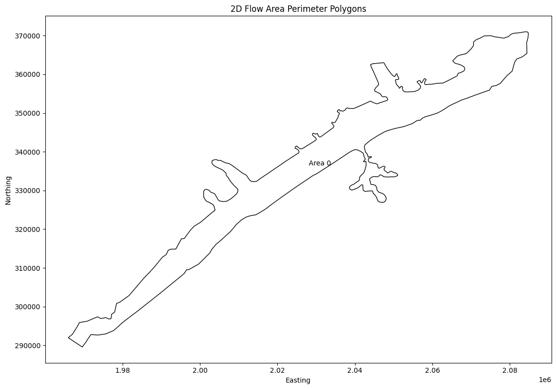
# Get 2D Flow Area Perimeter Polygons (get_mesh_areas)
print("\nExtracting 2D Flow Area Perimeter Polygons")
mesh_areas = HdfMesh.get_mesh_areas(geom_hdf_path)
Extracting 2D Flow Area Perimeter Polygons
| mesh_name | geometry | |
|---|---|---|
| 0 | BaldEagleCr | POLYGON ((2009315.708 321138.385, 2009371.858 ... |
# Generate Map of Mesh Areas
if generate_plots:
    # Plot the 2D Flow Area Perimeter Polygons
    import matplotlib.pyplot as plt

    fig, ax = plt.subplots(figsize=(12, 8))
    mesh_areas.plot(ax=ax, edgecolor='black', facecolor='none')

    # Add labels for each polygon
    for idx, row in mesh_areas.iterrows():
        centroid = row.geometry.centroid
        # Check if 'Name' column exists, otherwise use a default label
        label = row.get('Name', f'Area {idx}')
        ax.annotate(label, (centroid.x, centroid.y), ha='center', va='center')

    plt.title('2D Flow Area Perimeter Polygons')
    plt.xlabel('Easting')
    plt.ylabel('Northing')
    plt.tight_layout()
    plt.show()
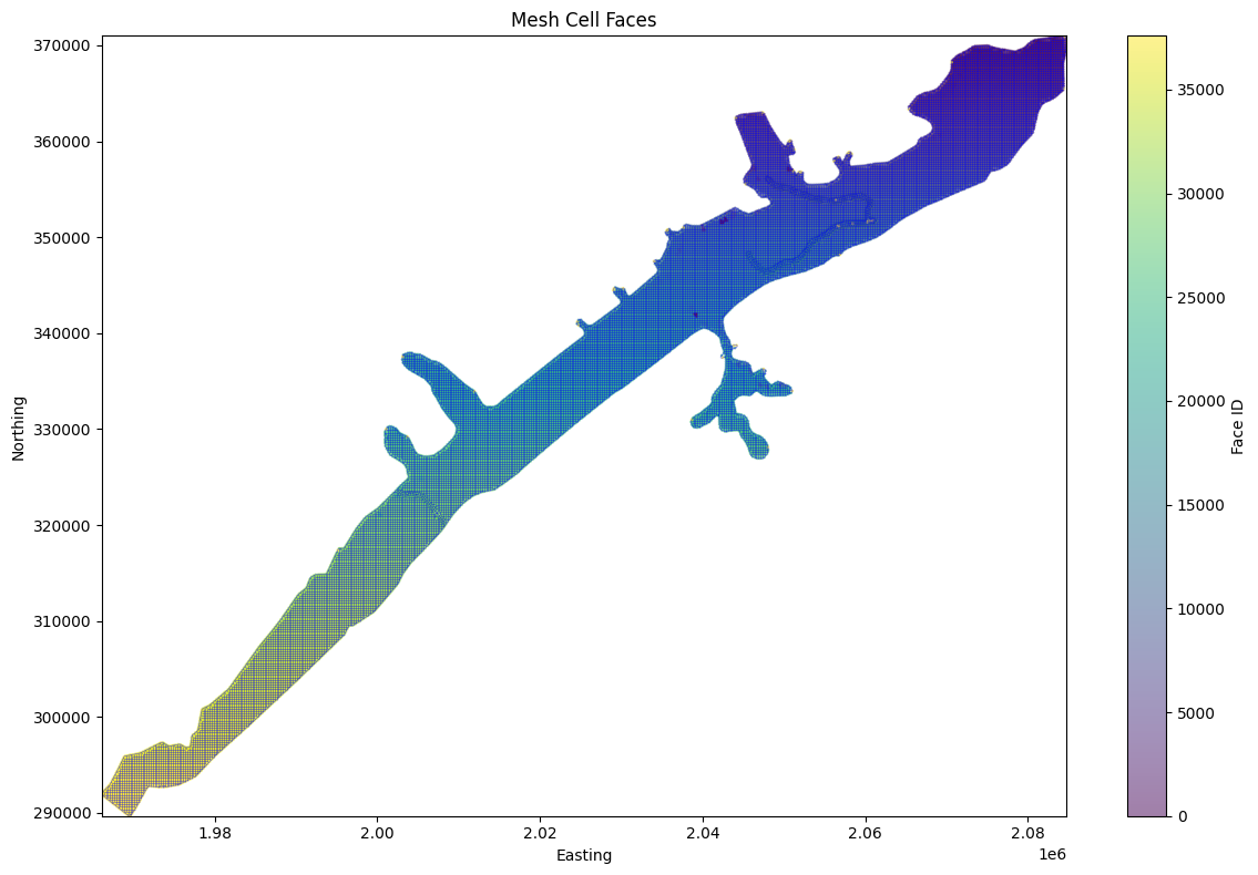
# Get mesh cell faces as geodatframe
mesh_cell_faces_gdf = HdfMesh.get_mesh_cell_faces(geom_hdf_path)
| mesh_name | face_id | geometry | |
|---|---|---|---|
| 0 | BaldEagleCr | 0 | LINESTRING (2042125 351625, 2042375 351625) |
| 1 | BaldEagleCr | 1 | LINESTRING (2042375 351625, 2042375 351875) |
| 2 | BaldEagleCr | 2 | LINESTRING (2042375 351875, 2042125 351875) |
| 3 | BaldEagleCr | 3 | LINESTRING (2042125 351875, 2042125 351625) |
| 4 | BaldEagleCr | 4 | LINESTRING (2042375 351375, 2042375 351625) |
| ... | ... | ... | ... |
| 37589 | BaldEagleCr | 37589 | LINESTRING (1978444.054 300812.794, 1978402.01... |
| 37590 | BaldEagleCr | 37590 | LINESTRING (1973531.76 297370.846, 1973246.989... |
| 37591 | BaldEagleCr | 37591 | LINESTRING (1968886.801 295900.5, 1968782.778 ... |
| 37592 | BaldEagleCr | 37592 | LINESTRING (1965981.775 291978.68, 1966280.11 ... |
| 37593 | BaldEagleCr | 37593 | LINESTRING (1969588.438 289578.114, 1969731.65... |
37594 rows × 3 columns
from matplotlib.collections import LineCollection
import numpy as np

# Calculate and display statistics
print("\nMesh Cell Faces Statistics:")
print(f"Total number of cell faces: {len(mesh_cell_faces_gdf)}")
print(f"Number of unique meshes: {mesh_cell_faces_gdf['mesh_name'].nunique()}")

if generate_maps:
    # Plot the mesh cell faces more efficiently
    fig, ax = plt.subplots(figsize=(12, 8))

    # Convert all geometries to numpy arrays at once for faster plotting
    lines = [list(zip(*line.xy)) for line in mesh_cell_faces_gdf.geometry]
    lines_collection = LineCollection(lines, colors='blue', linewidth=0.5, alpha=0.5)
    ax.add_collection(lines_collection)

    # Set plot title and labels
    plt.title('Mesh Cell Faces')
    plt.xlabel('Easting')
    plt.ylabel('Northing')

    # Calculate centroids once and store as numpy arrays
    centroids = np.array([[geom.centroid.x, geom.centroid.y] for geom in mesh_cell_faces_gdf.geometry])

    # Create scatter plot with numpy arrays
    scatter = ax.scatter(
        centroids[:, 0],
        centroids[:, 1],
        c=mesh_cell_faces_gdf['face_id'],
        cmap='viridis',
        s=1,
        alpha=0.5
    )
    plt.colorbar(scatter, label='Face ID')

    # Set axis limits based on data bounds
    ax.set_xlim(centroids[:, 0].min(), centroids[:, 0].max())
    ax.set_ylim(centroids[:, 1].min(), centroids[:, 1].max())

    plt.tight_layout()
    plt.show()
else:
    print("generate_maps is False")
Mesh Cell Faces Statistics:
Total number of cell faces: 37594
Number of unique meshes: 1
# Example: Find the nearest cell face to a given point using library API
# The HdfMesh.find_nearest_face() function replaces the notebook's custom helper

print("\nExample: Finding the nearest cell face to a given point")

from shapely.geometry import Point
import geopandas as gpd

# Ensure mesh_cell_faces_gdf exists from previous cell
if 'mesh_cell_faces_gdf' in dir() and not mesh_cell_faces_gdf.empty:
    # Create a deterministic sample point inside the project extent.
    representative_face = mesh_cell_faces_gdf.geometry.iloc[len(mesh_cell_faces_gdf) // 2]
    representative_centroid = representative_face.centroid
    sample_coords = (representative_centroid.x + 50.0, representative_centroid.y + 50.0)

    # Use library API to find nearest face
    # HdfMesh.find_nearest_face(point, cell_faces_gdf, mesh_name=None) -> (face_id, distance)
    nearest_face_id, distance = HdfMesh.find_nearest_face(sample_coords, mesh_cell_faces_gdf)

    print(f"Nearest cell face to point {sample_coords}:")
    print(f"Face ID: {nearest_face_id}")
    print(f"Distance: {distance:.2f} units")

    # Visualize the result
    if nearest_face_id is not None:
        fig, ax = plt.subplots(figsize=(12, 8))

        # Plot the sample point
        sample_point_gdf = gpd.GeoDataFrame(
            {'geometry': [Point(sample_coords)]},
            crs=mesh_cell_faces_gdf.crs
        )
        # Plot the nearest cell face
        nearest_face = mesh_cell_faces_gdf[mesh_cell_faces_gdf['face_id'] == nearest_face_id]
        nearest_geom = nearest_face.geometry.iloc[0]
        xmin, ymin, xmax, ymax = nearest_geom.union(sample_point_gdf.geometry.iloc[0]).bounds
        plot_margin = max(distance * 2.0, nearest_geom.length * 2.0, 250.0)
        local_window = mesh_cell_faces_gdf.cx[
            xmin - plot_margin:xmax + plot_margin,
            ymin - plot_margin:ymax + plot_margin,
        ]

        # Plot nearby cell faces so the nearest-face relationship is readable.
        local_window.plot(ax=ax, color='lightgray', linewidth=0.8, alpha=0.8, label='Nearby Cell Faces')
        nearest_face.plot(ax=ax, color='green', linewidth=3, alpha=0.9, label='Nearest Face')
        sample_point_gdf.plot(ax=ax, color='red', markersize=100, alpha=0.8, label='Sample Point')

        # Set labels and title
        ax.set_xlim(xmin - plot_margin, xmax + plot_margin)
        ax.set_ylim(ymin - plot_margin, ymax + plot_margin)
        ax.set_aspect('equal', adjustable='box')
        ax.set_xlabel('Project X Coordinate (ft)')
        ax.set_ylabel('Project Y Coordinate (ft)')
        ax.set_title(f'Nearest Cell Face to Sample Point (distance = {distance:.1f} ft)')

        # Add legend and grid
        ax.legend()
        ax.grid(True)

        plt.tight_layout()
        plt.show()
else:
    print("Note: mesh_cell_faces_gdf not available - run mesh cell faces extraction cell first")
Example: Finding the nearest cell face to a given point
Nearest cell face to point (2035175.0, 339300.0):
Face ID: 18797
Distance: 50.00 units
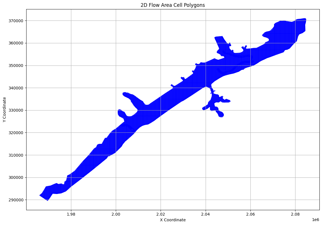
# Extract Cell Polygons
print("\nExample 6: Extracting Cell Polygons")
cell_polygons_df = HdfMesh.get_mesh_cell_polygons(geom_hdf_path)
Example 6: Extracting Cell Polygons
| mesh_name | cell_id | geometry | |
|---|---|---|---|
| 0 | BaldEagleCr | 0 | POLYGON ((2082875 370625, 2082723.922 370776.0... |
| 1 | BaldEagleCr | 1 | POLYGON ((2083125 370625, 2083125 370844.185, ... |
| 2 | BaldEagleCr | 2 | POLYGON ((2083375 370625, 2083375 370886.638, ... |
| 3 | BaldEagleCr | 3 | POLYGON ((2083625 370625, 2083625 370925.693, ... |
| 4 | BaldEagleCr | 4 | POLYGON ((2083875 370625, 2083875 370958.588, ... |
| ... | ... | ... | ... |
| 18061 | BaldEagleCr | 18061 | POLYGON ((2060605.501 351955.442, 2060652.06 3... |
| 18062 | BaldEagleCr | 18062 | POLYGON ((2060652.06 351777.237, 2060849.045 3... |
| 18063 | BaldEagleCr | 18063 | POLYGON ((2060875 351951.343, 2060929.66 35193... |
| 18064 | BaldEagleCr | 18064 | POLYGON ((2060991.954 351624.893, 2060964.72 3... |
| 18065 | BaldEagleCr | 18065 | POLYGON ((2061172.274 351856.061, 2061298.822 ... |
18066 rows × 3 columns
# Plot cell polygons

if generate_maps:
    fig, ax = plt.subplots(figsize=(12, 8))

    # Plot cell polygons
    cell_polygons_df.plot(ax=ax, edgecolor='blue', facecolor='none')

    # Set labels and title
    ax.set_xlabel('X Coordinate')
    ax.set_ylabel('Y Coordinate')
    ax.set_title('2D Flow Area Cell Polygons')

    # Add grid
    ax.grid(True)

    # Adjust layout and display
    plt.tight_layout()
    plt.show()
else:
    print("generate_maps is set to False")
# Extract Cell Info
print("\nExample 5: Extracting Cell Info")
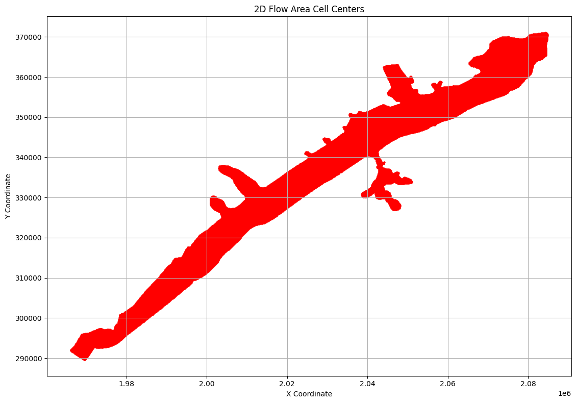
cell_info_df = HdfMesh.get_mesh_cell_points(geom_hdf_path)
Example 5: Extracting Cell Info
| mesh_name | cell_id | geometry | |
|---|---|---|---|
| 0 | BaldEagleCr | 0 | POINT (2083000 370750) |
| 1 | BaldEagleCr | 1 | POINT (2083250 370750) |
| 2 | BaldEagleCr | 2 | POINT (2083500 370750) |
| 3 | BaldEagleCr | 3 | POINT (2083750 370750) |
| 4 | BaldEagleCr | 4 | POINT (2084000 370750) |
| ... | ... | ... | ... |
| 19592 | BaldEagleCr | 19592 | POINT (1978423.032 300718.897) |
| 19593 | BaldEagleCr | 19593 | POINT (1973389.375 297311.928) |
| 19594 | BaldEagleCr | 19594 | POINT (1968834.79 295808.861) |
| 19595 | BaldEagleCr | 19595 | POINT (1966130.942 291879.395) |
| 19596 | BaldEagleCr | 19596 | POINT (1969660.046 289673.23) |
19597 rows × 3 columns
# Plot cell centers

if generate_maps:
    fig, ax = plt.subplots(figsize=(12, 8))

    # Plot cell centers
    cell_info_df.plot(ax=ax, color='red', markersize=5)

    # Set labels and title
    ax.set_xlabel('X Coordinate')
    ax.set_ylabel('Y Coordinate')
    ax.set_title('2D Flow Area Cell Centers')

    # Add grid
    ax.grid(True)

    # Adjust layout and display
    plt.tight_layout()
    plt.show()
else:
    print("generate_maps is set to False")
# Get geometry structures attributes
print("\nGetting geometry structures attributes as Dataframe")
geom_structures_attrs = HdfStruc.get_geom_structures_attrs(geom_hdf_path)
Getting geometry structures attributes as Dataframe
| Bridge/Culvert Count | Connection Count | Has Bridge Opening (2D) | Inline Structure Count | Lateral Structure Count | |
|---|---|---|---|---|---|
| 0 | 0 | 1 | 0 | 0 | 0 |
# TODO: Paths and Functions for each type of structure:

# Getting geometry structures attributes
# Geometry structures attributes:
# Bridge/Culvert Count: 0
# Connection Count: 4
# Has Bridge Opening (2D): 0
# Inline Structure Count: 0
# Lateral Structure Count: 0
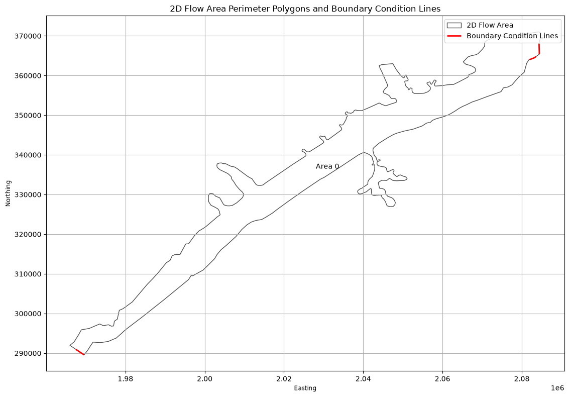
# Get boundary condition lines
print("\nExtracting Boundary Condition Lines as Geodataframe")
bc_lines_df = HdfBndry.get_bc_lines(geom_hdf_path)
Extracting Boundary Condition Lines as Geodataframe
| Name | SA-2D | Type | Length | geometry | bc_line_id | |
|---|---|---|---|---|---|---|
| 0 | DSNormalDepth | BaldEagleCr | External | 1801.303345 | LINESTRING (2082004.235 364024.82, 2083193.546... | 0 |
| 1 | DS2NormalD | BaldEagleCr | External | 2633.932617 | LINESTRING (2084425.804 365392.892, 2084354.64... | 1 |
| 2 | Upstream Inflow | BaldEagleCr | External | 2533.638672 | LINESTRING (1967473.737 290973.629, 1969582.89... | 2 |
# Plot Boundary Condition Lines with Perimeter

if generate_maps:
    fig, ax = plt.subplots(figsize=(12, 8))

    if not mesh_areas.empty:
        mesh_areas.plot(ax=ax, edgecolor='black', facecolor='none', alpha=0.7, label='2D Flow Area')

        # Add labels for each polygon
        for idx, row in mesh_areas.iterrows():
            centroid = row.geometry.centroid
            label = row.get('Name', f'Area {idx}')
            ax.annotate(label, (centroid.x, centroid.y), ha='center', va='center')

    # Plot boundary condition lines
    if not bc_lines_df.empty:
        bc_lines_df.plot(ax=ax, color='red', linewidth=2, label='Boundary Condition Lines')

    # Set labels and title
    ax.set_xlabel('Easting')
    ax.set_ylabel('Northing')
    ax.set_title('2D Flow Area Perimeter Polygons and Boundary Condition Lines')

    # Add grid and legend
    ax.grid(True)
    ax.legend()

    # Adjust layout and display
    plt.tight_layout()
    plt.show()

else:
    print("generate_maps is set to False")
# Plot 2D Flow Area Perimeter Polygons
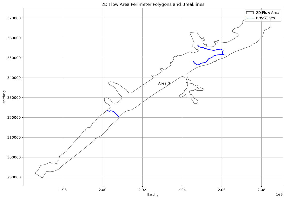
# Extract Breaklines as Geodataframe
print("\nExtracting Breaklines")
breaklines_gdf = HdfBndry.get_breaklines(geom_hdf_path)
Extracting Breaklines
| bl_id | Name | cell_spacing_near | cell_spacing_far | near_repeats | protection_radius | geometry | |
|---|---|---|---|---|---|---|---|
| 0 | 0 | SayersDam | NaN | NaN | 0 | 0 | LINESTRING (2002361.246 323707.927, 2002741.35... |
| 1 | 1 | Lower | NaN | NaN | 0 | 0 | LINESTRING (2060356.422 351786.819, 2060316.47... |
| 2 | 2 | Middle | NaN | NaN | 0 | 0 | LINESTRING (2052757.788 348470.547, 2052785.84... |
| 3 | 3 | Upper | NaN | NaN | 0 | 0 | LINESTRING (2045597.199 348412.994, 2045638.91... |
# Plot breaklines and 2D Flow Area Perimeter Polygons

if generate_plots:
    fig, ax = plt.subplots(figsize=(12, 8))

    # Plot 2D Flow Area Perimeter Polygons
    if not mesh_areas.empty:
        mesh_areas.plot(ax=ax, edgecolor='black', facecolor='none', alpha=0.7, label='2D Flow Area')

        # Add labels for each polygon
        for idx, row in mesh_areas.iterrows():
            centroid = row.geometry.centroid
            label = row.get('Name', f'Area {idx}')
            ax.annotate(label, (centroid.x, centroid.y), ha='center', va='center')

    # Plot breaklines
    if not breaklines_gdf.empty:
        breaklines_gdf.plot(ax=ax, color='blue', linewidth=2, label='Breaklines')

    # Set labels and title
    ax.set_xlabel('Easting')
    ax.set_ylabel('Northing')
    ax.set_title('2D Flow Area Perimeter Polygons and Breaklines')

    # Add grid and legend
    ax.grid(True)
    ax.legend()

    # Adjust layout and display
    plt.tight_layout()
    plt.show()
| Type | Mode | River | Reach | RS | Connection | Groupname | US Type | US River | US Reach | ... | US XS Mann (Count) | US BR Mann (Index) | US BR Mann (Count) | DS XS Mann (Index) | DS XS Mann (Count) | DS BR Mann (Index) | DS BR Mann (Count) | RC (Index) | RC (Count) | Profile_Data | |
|---|---|---|---|---|---|---|---|---|---|---|---|---|---|---|---|---|---|---|---|---|---|
| 0 | Connection | Weir/Gate/Culverts | Sayers Dam | BaldEagleCr, Sayers Dam | 2D | ... | 0 | 0 | 0 | 0 | 0 | 0 | 0 | 0 | 0 | [{'Station': 0.0, 'Elevation': 683.0}, {'Stati... |
1 rows × 163 columns
# Get boundary condition lines as GeoDatframe
bc_lines_gdf = HdfBndry.get_bc_lines(geom_hdf_path)
print("\nBoundary Condition Lines:")
Boundary Condition Lines:
| Name | SA-2D | Type | Length | geometry | bc_line_id | |
|---|---|---|---|---|---|---|
| 0 | DSNormalDepth | BaldEagleCr | External | 1801.303345 | LINESTRING (2082004.235 364024.82, 2083193.546... | 0 |
| 1 | DS2NormalD | BaldEagleCr | External | 2633.932617 | LINESTRING (2084425.804 365392.892, 2084354.64... | 1 |
| 2 | Upstream Inflow | BaldEagleCr | External | 2533.638672 | LINESTRING (1967473.737 290973.629, 1969582.89... | 2 |
Dev Note: Need to add function for Reference Lines
# Get reference points as Geodataframe
ref_points_gdf = HdfBndry.get_reference_points(geom_hdf_path)
print("\nReference Points:")
ref_points_gdf
# There are no reference points in this example project (for demonstration only)
Reference Points:
# Extract Refinement Regions
refinement_regions_df = HdfBndry.get_refinement_regions(geom_hdf_path)
# Plot Refinement Regions

if not refinement_regions_df.empty:
    print("Refinement Regions DataFrame:")
    display(refinement_regions_df.head())

    # Plot refinement regions
    fig, ax = plt.subplots(figsize=(12, 8))
    refinement_regions_df.plot(ax=ax, column='CellSize', legend=True,
                               legend_kwds={'label': 'Cell Size', 'orientation': 'horizontal'},
                               cmap='viridis')
    ax.set_title('2D Mesh Area Refinement Regions')
    ax.set_xlabel('Easting')
    ax.set_ylabel('Northing')
    plt.tight_layout()
    plt.show()
else:
    print("No refinement regions found in the geometry file.")

# Analyze Refinement Regions
if not refinement_regions_df.empty:
    print("\nRefinement Regions Analysis:")
    print(f"Total number of refinement regions: {len(refinement_regions_df)}")
    print("\nCell Size Statistics:")
    print(refinement_regions_df['CellSize'].describe())

    # Group by Shape Type
    shape_type_counts = refinement_regions_df['ShapeType'].value_counts()
    print("\nRefinement Region Shape Types:")
    print(shape_type_counts)

    # Plot Shape Type distribution
    plt.figure(figsize=(10, 6))
    shape_type_counts.plot(kind='bar')
    plt.title('Distribution of Refinement Region Shape Types')
    plt.xlabel('Shape Type')
    plt.ylabel('Count')
    plt.xticks(rotation=45)
    plt.tight_layout()
    plt.show()
No refinement regions found in the geometry file.
| Plan | Parameter | Value | |
|---|---|---|---|
| 0 | 06 | 1D Cores | 2 |
| 1 | 06 | 1D Flow Tolerance | NaN |
| 2 | 06 | 1D Maximum Iterations | 20 |
| 3 | 06 | 1D Maximum Iterations Without Improvement | 0 |
| 4 | 06 | 1D Maximum Water Surface Error To Abort | 100.0 |
| 5 | 06 | 1D Methodology | Finite Difference |
| 6 | 06 | 1D Storage Area Elevation Tolerance | 0.02 |
| 7 | 06 | 1D Theta | 1.0 |
| 8 | 06 | 1D Theta Warmup | 1.0 |
| 9 | 06 | 1D Water Surface Elevation Tolerance | 0.02 |
| 10 | 06 | 1D-2D Flow Tolerance | 1.0 |
| 11 | 06 | 1D-2D Gate Flow Submergence Decay Exponent | 1.0 |
| 12 | 06 | 1D-2D IS Stablity Factor | 1.0 |
| 13 | 06 | 1D-2D LS Stablity Factor | 2.0 |
| 14 | 06 | 1D-2D Maximum Iterations | 0 |
| 15 | 06 | 1D-2D Maximum Number of Time Slices | 20 |
| 16 | 06 | 1D-2D Minimum Flow Tolerance | NaN |
| 17 | 06 | 1D-2D Minimum Time Step for Slicing(hours) | 0.0 |
| 18 | 06 | 1D-2D Number of Warmup Steps | 0 |
| 19 | 06 | 1D-2D Warmup Time Step (hours) | 0.0 |
| 20 | 06 | 1D-2D Water Surface Tolerance | 0.02 |
| 21 | 06 | 1D-2D Weir Flow Submergence Decay Exponent | 1.0 |
| 22 | 06 | 2D Advanced Convergence | 0 |
| 23 | 06 | 2D Boundary Condition Ramp Up Fraction | 0.5 |
| 24 | 06 | 2D Boundary Condition Volume Check | False |
| 25 | 06 | 2D Cores (per mesh) | 2 |
| 26 | 06 | 2D Coriolis | False |
| 27 | 06 | 2D Equation Set | Diffusion Wave |
| 28 | 06 | 2D Initial Conditions Ramp Up Time (hrs) | 0.0 |
| 29 | 06 | 2D Latitude for Coriolis | 340282346638528859811704183484516925440.0 |
| 30 | 06 | 2D Longitudinal Mixing Coefficient | 0.0 |
| 31 | 06 | 2D Matrix Solver | Pardiso |
| 32 | 06 | 2D Maximum Iterations | 20 |
| 33 | 06 | 2D Names | BaldEagleCr |
| 34 | 06 | 2D Number of Time Slices | 1 |
| 35 | 06 | 2D Only | True |
| 36 | 06 | 2D Smagorinsky Mixing Coefficient | 0.0 |
| 37 | 06 | 2D Theta | 1.0 |
| 38 | 06 | 2D Theta Warmup | 1.0 |
| 39 | 06 | 2D Transverse Mixing Coefficient | 0.0 |
| 40 | 06 | 2D Turbulence Formulation | None |
| 41 | 06 | 2D Volume Tolerance | 0.01 |
| 42 | 06 | 2D WS Max Tolerance | 0.0 |
| 43 | 06 | 2D WS RMS Tolerance | 0.0 |
| 44 | 06 | 2D WS Stalling Tolerance | 0.0 |
| 45 | 06 | 2D Water Surface Tolerance | 0.01 |
| 46 | 06 | Friction Slope Average Method (BR) | Average Conveyance |
| 47 | 06 | Friction Slope Average Method (XS) | Average Friction Slope |
| 48 | 06 | Gravity | 32.174 |
| 49 | 06 | HDF Additional Output Variables | [Cell Velocity, Face Eddy Viscosity, Face Flow... |
| 50 | 06 | HDF Chunk Size | 1.0 |
| 51 | 06 | HDF Compression | 1 |
| 52 | 06 | HDF Fixed Rows | 1 |
| 53 | 06 | HDF Flush Buffer | False |
| 54 | 06 | HDF Spatial Parts | 1 |
| 55 | 06 | HDF Use Max Rows | 0 |
| 56 | 06 | HDF Write Time Slices | False |
| 57 | 06 | HDF Write Warmup | False |
| 58 | 06 | Pardiso Solver | False |
| 59 | 06 | Reproducibility Mode | 0 |
# Extract volume accounting data
volume_accounting_df = HdfResultsPlan.get_volume_accounting(plan_hdf_path)
| Error | Error Percent | Precipitation Excess (acre feet) | Precipitation Excess (inches) | Total Boundary Flux of Water In | Total Boundary Flux of Water Out | Vol Accounting in | Volume Ending | Volume Starting | |
|---|---|---|---|---|---|---|---|---|---|
| 0 | 0.610979 | 0.000431 | 3756.872803 | 1.707615 | 141685.265625 | 17253.21875 | Acre Feet | 124432.664062 | 0.0 |
RasPlanHdf Class Functions
# Get plan start time as datetime object
start_time = HdfPlan.get_plan_start_time(plan_hdf_path)
print(f"Simulation start time: {start_time}")
Simulation start time: 2018-09-09 00:00:00
Simulation start time: 2018-09-09 00:00:00
# Get plan end time as datetime object
end_time = HdfPlan.get_plan_end_time(plan_hdf_path)
print(f"Simulation end time: {end_time}")
Simulation end time: 2018-09-14 00:00:00
Simulation end time: 2018-09-14 00:00:00
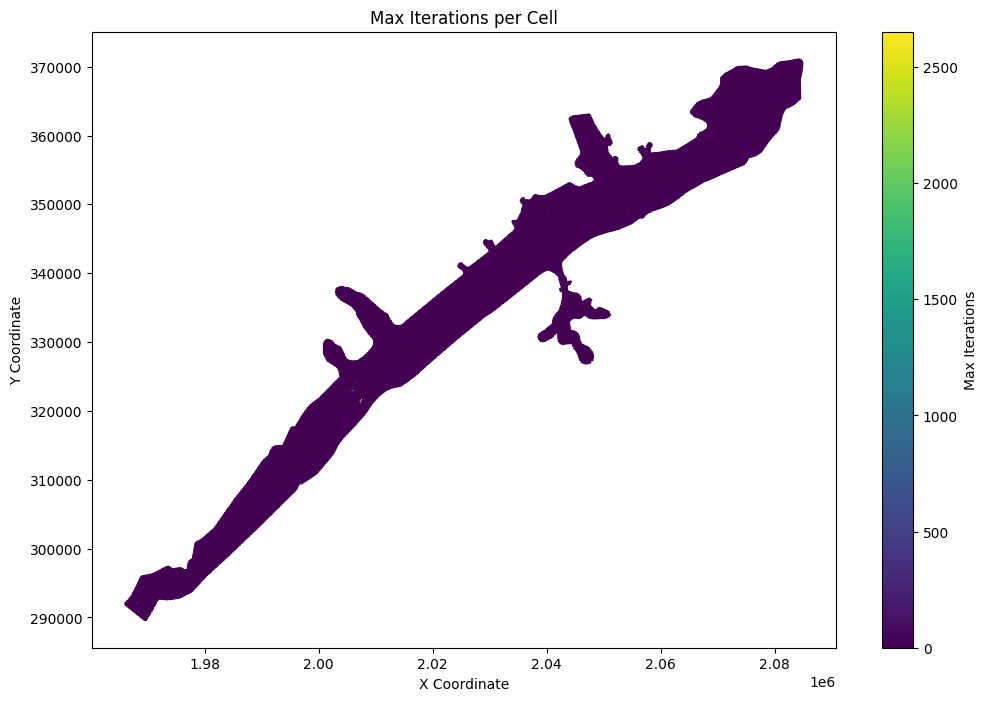
# Get maximum iteration count for mesh cells
max_iter_gdf = HdfResultsMesh.get_mesh_max_iter(plan_hdf_path)
| mesh_name | cell_id | cell_last_iteration | is_ghost_cell | geometry | |
|---|---|---|---|---|---|
| 0 | BaldEagleCr | 0 | 0 | False | POINT (2083000 370750) |
| 1 | BaldEagleCr | 1 | 2 | False | POINT (2083250 370750) |
| 2 | BaldEagleCr | 2 | 0 | False | POINT (2083500 370750) |
| 3 | BaldEagleCr | 3 | 0 | False | POINT (2083750 370750) |
| 4 | BaldEagleCr | 4 | 0 | False | POINT (2084000 370750) |
| ... | ... | ... | ... | ... | ... |
| 18061 | BaldEagleCr | 18061 | 0 | False | POINT (2060527.525 351824.248) |
| 18062 | BaldEagleCr | 18062 | 0 | False | POINT (2060770.734 351834.938) |
| 18063 | BaldEagleCr | 18063 | 0 | False | POINT (2060928.42 351836.275) |
| 18064 | BaldEagleCr | 18064 | 0 | False | POINT (2061024.634 351710.661) |
| 18065 | BaldEagleCr | 18065 | 0 | False | POINT (2061115.504 351702.643) |
18066 rows × 5 columns
# Plot Mesh Max Iterations

if generate_maps:
    # Extract x and y coordinates from the geometry column
    max_iter_gdf['x'] = max_iter_gdf['geometry'].apply(lambda geom: geom.x if geom is not None else None)
    max_iter_gdf['y'] = max_iter_gdf['geometry'].apply(lambda geom: geom.y if geom is not None else None)

    # Remove rows with None coordinates
    max_iter_gdf = max_iter_gdf.dropna(subset=['x', 'y'])

    # Create the plot
    fig, ax = plt.subplots(figsize=(12, 8))
    scatter = ax.scatter(max_iter_gdf['x'], max_iter_gdf['y'],
                         c=max_iter_gdf['cell_last_iteration'],
                         cmap='viridis',
                         s=1)

    # Customize the plot
    ax.set_title('Max Iterations per Cell')
    ax.set_xlabel('X Coordinate')
    ax.set_ylabel('Y Coordinate')
    plt.colorbar(scatter, label='Max Iterations')

    # Show the plot
    plt.show()
else:
    print("generate_maps is set to False")

# Print the first few rows of the dataframe for verification
print("\nFirst few rows of the dataframe:")
max_iter_gdf[['mesh_name', 'cell_id', 'geometry']]
First few rows of the dataframe:
| mesh_name | cell_id | geometry | |
|---|---|---|---|
| 0 | BaldEagleCr | 0 | POINT (2083000 370750) |
| 1 | BaldEagleCr | 1 | POINT (2083250 370750) |
| 2 | BaldEagleCr | 2 | POINT (2083500 370750) |
| 3 | BaldEagleCr | 3 | POINT (2083750 370750) |
| 4 | BaldEagleCr | 4 | POINT (2084000 370750) |
| ... | ... | ... | ... |
| 18061 | BaldEagleCr | 18061 | POINT (2060527.525 351824.248) |
| 18062 | BaldEagleCr | 18062 | POINT (2060770.734 351834.938) |
| 18063 | BaldEagleCr | 18063 | POINT (2060928.42 351836.275) |
| 18064 | BaldEagleCr | 18064 | POINT (2061024.634 351710.661) |
| 18065 | BaldEagleCr | 18065 | POINT (2061115.504 351702.643) |
18066 rows × 3 columns
# List top 10 points for Max Iteration per Cell
# Sort the dataframe by cell_last_iteration in descending order
top_iterations = max_iter_gdf.sort_values(by='cell_last_iteration', ascending=False).head(10)

# Create a more informative display with coordinates
print("\nTop 10 Cells with Highest Iteration Counts:")
top_iterations_display = top_iterations.copy()
top_iterations_display['x_coord'] = top_iterations_display['geometry'].apply(lambda geom: round(geom.x, 2))
top_iterations_display['y_coord'] = top_iterations_display['geometry'].apply(lambda geom: round(geom.y, 2))

# Display the results in a formatted table
print(top_iterations_display[['mesh_name', 'cell_id', 'cell_last_iteration', 'x_coord', 'y_coord']])
Top 10 Cells with Highest Iteration Counts:
         mesh_name  cell_id  cell_last_iteration     x_coord    y_coord
17721  BaldEagleCr    17721                 1223  2007386.39  321546.77
17752  BaldEagleCr    17752                  995  2005903.93  322873.01
17621  BaldEagleCr    17621                  509  1968250.00  292000.00
16970  BaldEagleCr    16970                  293  1973750.00  296500.00
13039  BaldEagleCr    13039                  202  2006750.00  324250.00
8749   BaldEagleCr     8749                  180  2028000.00  339000.00
14658  BaldEagleCr    14658                  179  1993500.00  314000.00
16643  BaldEagleCr    16643                  158  1981750.00  300000.00
13520  BaldEagleCr    13520                  157  2007000.00  321250.00
13978  BaldEagleCr    13978                  156  1997500.00  318250.00
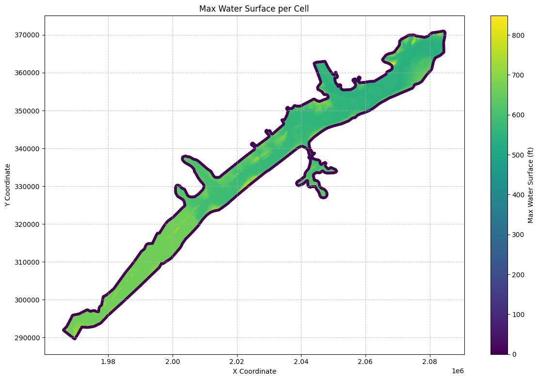
# Get mesh maximum water surface elevation as Geodataframe
max_ws_gdf = HdfResultsMesh.get_mesh_max_ws(plan_hdf_path)
# Check Dataframe Attributes (the HDF Attributes are also imported as Geoataframe Attributes)
max_ws_gdf.attrs
{'mesh_name': 'BaldEagleCr',
 'Max Time': np.float32(5.0),
 'Max Value': np.float32(848.20447),
 'Min Time': np.float32(1.0002315),
 'Min Value': np.float32(535.58484),
 'Rows Variables': ['WSEL', 'Time'],
 'Units': ['ft', 'days']}
| mesh_name | cell_id | maximum_water_surface | maximum_water_surface_time | is_ghost_cell | geometry | |
|---|---|---|---|---|---|---|
| 0 | BaldEagleCr | 0 | 704.053711 | 2018-09-10 18:00:00 | False | POINT (2083000 370750) |
| 1 | BaldEagleCr | 1 | 692.376953 | 2018-09-10 18:04:00 | False | POINT (2083250 370750) |
| 2 | BaldEagleCr | 2 | 671.182983 | 2018-09-10 18:13:00 | False | POINT (2083500 370750) |
| 3 | BaldEagleCr | 3 | 660.605042 | 2018-09-10 18:54:00 | False | POINT (2083750 370750) |
| 4 | BaldEagleCr | 4 | 660.585876 | 2018-09-10 18:55:40 | False | POINT (2084000 370750) |
| ... | ... | ... | ... | ... | ... | ... |
| 18061 | BaldEagleCr | 18061 | 550.542236 | 2018-09-10 19:00:00 | False | POINT (2060527.525 351824.248) |
| 18062 | BaldEagleCr | 18062 | 550.562988 | 2018-09-10 19:00:20 | False | POINT (2060770.734 351834.938) |
| 18063 | BaldEagleCr | 18063 | 550.590271 | 2018-09-10 19:00:00 | False | POINT (2060928.42 351836.275) |
| 18064 | BaldEagleCr | 18064 | 568.098022 | 2018-09-10 18:00:00 | False | POINT (2061024.634 351710.661) |
| 18065 | BaldEagleCr | 18065 | 551.708435 | 2018-09-10 09:57:00 | False | POINT (2061115.504 351702.643) |
18066 rows × 6 columns
# Plot the max water surface as a map
if generate_maps:
    # Extract x and y coordinates from the geometry column
    max_ws_gdf['x'] = max_ws_gdf['geometry'].apply(lambda geom: geom.x if geom is not None else None)
    max_ws_gdf['y'] = max_ws_gdf['geometry'].apply(lambda geom: geom.y if geom is not None else None)

    # Remove rows with None coordinates
    max_ws_gdf = max_ws_gdf.dropna(subset=['x', 'y'])

    # Create the plot
    fig, ax = plt.subplots(figsize=(12, 8))
    scatter = ax.scatter(max_ws_gdf['x'], max_ws_gdf['y'],
                         c=max_ws_gdf['maximum_water_surface'],
                         cmap='viridis',
                         s=10)

    # Customize the plot
    ax.set_title('Max Water Surface per Cell')
    ax.set_xlabel('X Coordinate')
    ax.set_ylabel('Y Coordinate')
    plt.colorbar(scatter, label='Max Water Surface (ft)')

    # Add grid lines
    ax.grid(True, linestyle='--', alpha=0.7)

    # Increase font size for better readability
    plt.rcParams.update({'font.size': 12})

    # Adjust layout to prevent cutting off labels
    plt.tight_layout()

    # Show the plot
    plt.show()
else:
    print("generate_maps is set to False")
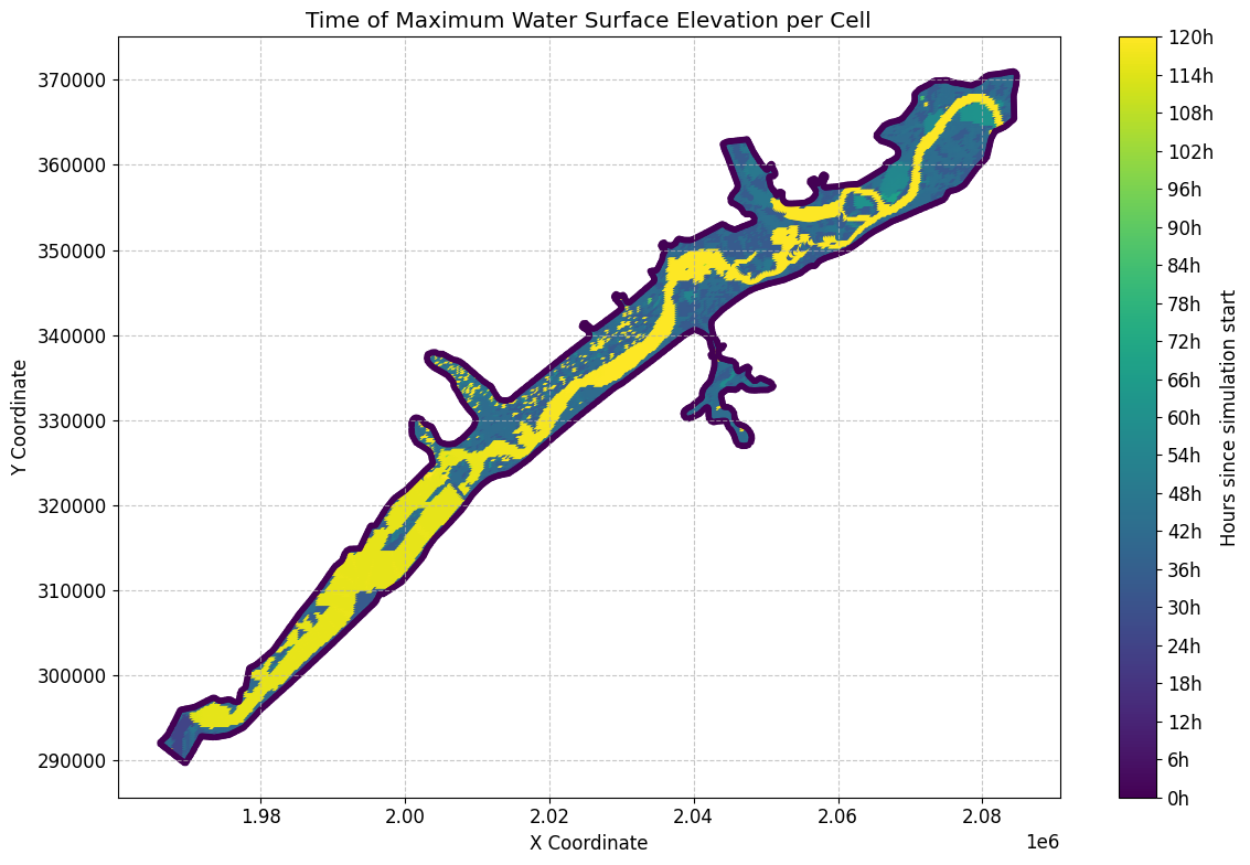
# Plot the time of the max water surface elevation (WSEL)
if generate_maps:
    import matplotlib.dates as mdates
    from datetime import datetime

    # Convert the 'maximum_water_surface_time' to datetime objects
    max_ws_gdf['max_wsel_time'] = pd.to_datetime(max_ws_gdf['maximum_water_surface_time'])

    # Create the plot
    fig, ax = plt.subplots(figsize=(12, 8))

    # Convert datetime to hours since the start for colormap
    min_time = max_ws_gdf['max_wsel_time'].min()
    color_values = (max_ws_gdf['max_wsel_time'] - min_time).dt.total_seconds() / 3600  # Convert to hours

    scatter = ax.scatter(max_ws_gdf['x'], max_ws_gdf['y'],
                        c=color_values,
                        cmap='viridis',
                        s=10)

    # Customize the plot
    ax.set_title('Time of Maximum Water Surface Elevation per Cell')
    ax.set_xlabel('X Coordinate')
    ax.set_ylabel('Y Coordinate')

    # Set up the colorbar
    cbar = plt.colorbar(scatter)
    cbar.set_label('Hours since simulation start')

    # Format the colorbar ticks to show hours
    cbar.set_ticks(range(0, int(color_values.max()) + 1, 6))  # Set ticks every 6 hours
    cbar.set_ticklabels([f'{h}h' for h in range(0, int(color_values.max()) + 1, 6)])

    # Add grid lines
    ax.grid(True, linestyle='--', alpha=0.7)

    # Increase font size for better readability
    plt.rcParams.update({'font.size': 12})

    # Adjust layout to prevent cutting off labels
    plt.tight_layout()

    # Show the plot
    plt.show()

    # Find the overall maximum WSEL and its time
    max_wsel_row = max_ws_gdf.loc[max_ws_gdf['maximum_water_surface'].idxmax()]
    hours_since_start = (max_wsel_row['max_wsel_time'] - min_time).total_seconds() / 3600
    print(f"\nOverall Maximum WSEL: {max_wsel_row['maximum_water_surface']:.2f} ft")
    print(f"Time of Overall Maximum WSEL: {max_wsel_row['max_wsel_time']}")
    print(f"Hours since simulation start: {hours_since_start:.2f} hours")
    print(f"Location of Overall Maximum WSEL: X={max_wsel_row['x']}, Y={max_wsel_row['y']}")
Overall Maximum WSEL: 848.20 ft
Time of Overall Maximum WSEL: 2018-09-10 17:00:00
Hours since simulation start: 16.99 hours
Location of Overall Maximum WSEL: X=1968500.0, Y=295000.0
# Get mesh minimum water surface elevation as geodataframe
min_ws_gdf = HdfResultsMesh.get_mesh_min_ws(plan_hdf_path)
| mesh_name | cell_id | minimum_water_surface | minimum_water_surface_time | is_ghost_cell | geometry | |
|---|---|---|---|---|---|---|
| 0 | BaldEagleCr | 0 | 701.151245 | 2018-09-09 00:00:20 | False | POINT (2083000 370750) |
| 1 | BaldEagleCr | 1 | 689.052246 | 2018-09-09 00:00:20 | False | POINT (2083250 370750) |
| 2 | BaldEagleCr | 2 | 669.774719 | 2018-09-09 00:00:20 | False | POINT (2083500 370750) |
| 3 | BaldEagleCr | 3 | 658.986938 | 2018-09-09 00:00:20 | False | POINT (2083750 370750) |
| 4 | BaldEagleCr | 4 | 658.720581 | 2018-09-09 00:00:20 | False | POINT (2084000 370750) |
| ... | ... | ... | ... | ... | ... | ... |
| 18061 | BaldEagleCr | 18061 | 550.192688 | 2018-09-09 00:00:20 | False | POINT (2060527.525 351824.248) |
| 18062 | BaldEagleCr | 18062 | 550.218750 | 2018-09-09 00:00:20 | False | POINT (2060770.734 351834.938) |
| 18063 | BaldEagleCr | 18063 | 550.218750 | 2018-09-09 00:00:20 | False | POINT (2060928.42 351836.275) |
| 18064 | BaldEagleCr | 18064 | 567.500488 | 2018-09-09 00:00:20 | False | POINT (2061024.634 351710.661) |
| 18065 | BaldEagleCr | 18065 | 551.280029 | 2018-09-09 00:00:20 | False | POINT (2061115.504 351702.643) |
18066 rows × 6 columns
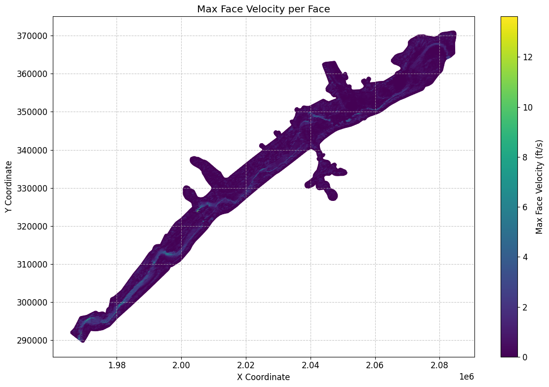
# Get mesh maximum face velocity as geodataframe
max_face_v_gdf = HdfResultsMesh.get_mesh_max_face_v(plan_hdf_path)
print("\nMesh Max Face Velocity:")
Mesh Max Face Velocity:
| mesh_name | face_id | maximum_face_velocity | maximum_face_velocity_time | geometry | |
|---|---|---|---|---|---|
| 0 | BaldEagleCr | 0 | 0.451467 | 2018-09-10 18:00:00 | LINESTRING (2042125 351625, 2042375 351625) |
| 1 | BaldEagleCr | 1 | -0.886932 | 2018-09-10 18:00:20 | LINESTRING (2042375 351625, 2042375 351875) |
| 2 | BaldEagleCr | 2 | -0.498507 | 2018-09-10 18:00:20 | LINESTRING (2042375 351875, 2042125 351875) |
| 3 | BaldEagleCr | 3 | -0.304597 | 2018-09-10 18:00:20 | LINESTRING (2042125 351875, 2042125 351625) |
| 4 | BaldEagleCr | 4 | -0.762412 | 2018-09-10 10:00:20 | LINESTRING (2042375 351375, 2042375 351625) |
| ... | ... | ... | ... | ... | ... |
| 37589 | BaldEagleCr | 37589 | 0.000000 | 2018-09-09 00:00:00 | LINESTRING (1978444.054 300812.794, 1978402.01... |
| 37590 | BaldEagleCr | 37590 | 0.000000 | 2018-09-09 00:00:00 | LINESTRING (1973531.76 297370.846, 1973246.989... |
| 37591 | BaldEagleCr | 37591 | 0.000000 | 2018-09-09 00:00:00 | LINESTRING (1968886.801 295900.5, 1968782.778 ... |
| 37592 | BaldEagleCr | 37592 | 0.000000 | 2018-09-09 00:00:00 | LINESTRING (1965981.775 291978.68, 1966280.11 ... |
| 37593 | BaldEagleCr | 37593 | 0.000000 | 2018-09-09 00:00:00 | LINESTRING (1969588.438 289578.114, 1969731.65... |
37594 rows × 5 columns
# Extract midpoint coordinates from the LineString geometries
max_face_v_gdf['x'] = max_face_v_gdf['geometry'].apply(lambda geom: geom.centroid.x)
max_face_v_gdf['y'] = max_face_v_gdf['geometry'].apply(lambda geom: geom.centroid.y)

# Create the plot
fig, ax = plt.subplots(figsize=(12, 8))
scatter = ax.scatter(max_face_v_gdf['x'], max_face_v_gdf['y'],
                    c=max_face_v_gdf['maximum_face_velocity'].abs(),
                    cmap='viridis',
                    s=10)

# Customize the plot
ax.set_title('Max Face Velocity per Face')
ax.set_xlabel('X Coordinate')
ax.set_ylabel('Y Coordinate')
plt.colorbar(scatter, label='Max Face Velocity (ft/s)')

# Add grid lines
ax.grid(True, linestyle='--', alpha=0.7)

# Increase font size for better readability
plt.rcParams.update({'font.size': 12})

# Adjust layout to prevent cutting off labels
plt.tight_layout()

# Show the plot
plt.show()
# Get mesh minimum face velocity as geodataframe
min_face_v_gdf = HdfResultsMesh.get_mesh_min_face_v(plan_hdf_path)
Mesh Min Face Velocity:
| mesh_name | face_id | minimum_face_velocity | minimum_face_velocity_time | geometry | |
|---|---|---|---|---|---|
| 0 | BaldEagleCr | 0 | 0.0 | 2018-09-09 00:00:20 | LINESTRING (2042125 351625, 2042375 351625) |
| 1 | BaldEagleCr | 1 | 0.0 | 2018-09-09 00:00:20 | LINESTRING (2042375 351625, 2042375 351875) |
| 2 | BaldEagleCr | 2 | 0.0 | 2018-09-09 00:00:20 | LINESTRING (2042375 351875, 2042125 351875) |
| 3 | BaldEagleCr | 3 | 0.0 | 2018-09-09 00:00:20 | LINESTRING (2042125 351875, 2042125 351625) |
| 4 | BaldEagleCr | 4 | 0.0 | 2018-09-09 00:00:20 | LINESTRING (2042375 351375, 2042375 351625) |
| ... | ... | ... | ... | ... | ... |
| 37589 | BaldEagleCr | 37589 | 0.0 | 2018-09-09 00:00:20 | LINESTRING (1978444.054 300812.794, 1978402.01... |
| 37590 | BaldEagleCr | 37590 | 0.0 | 2018-09-09 00:00:20 | LINESTRING (1973531.76 297370.846, 1973246.989... |
| 37591 | BaldEagleCr | 37591 | 0.0 | 2018-09-09 00:00:20 | LINESTRING (1968886.801 295900.5, 1968782.778 ... |
| 37592 | BaldEagleCr | 37592 | 0.0 | 2018-09-09 00:00:20 | LINESTRING (1965981.775 291978.68, 1966280.11 ... |
| 37593 | BaldEagleCr | 37593 | 0.0 | 2018-09-09 00:00:20 | LINESTRING (1969588.438 289578.114, 1969731.65... |
37594 rows × 5 columns
# Get mesh max water surface error as geodataframe

max_ws_err_gdf = HdfResultsMesh.get_mesh_max_ws_err(plan_hdf_path)
Mesh Max Water Surface Error:
| mesh_name | cell_id | cell_maximum_water_surface_error | cell_maximum_water_surface_error_time | is_ghost_cell | geometry | |
|---|---|---|---|---|---|---|
| 0 | BaldEagleCr | 0 | 0.000920 | 2018-09-10 22:24:20 | False | POINT (2083000 370750) |
| 1 | BaldEagleCr | 1 | 0.001439 | 2018-09-10 22:24:20 | False | POINT (2083250 370750) |
| 2 | BaldEagleCr | 2 | 0.003429 | 2018-09-10 09:11:20 | False | POINT (2083500 370750) |
| 3 | BaldEagleCr | 3 | 0.000620 | 2018-09-10 22:24:20 | False | POINT (2083750 370750) |
| 4 | BaldEagleCr | 4 | 0.002828 | 2018-09-10 09:09:40 | False | POINT (2084000 370750) |
| ... | ... | ... | ... | ... | ... | ... |
| 18061 | BaldEagleCr | 18061 | 0.000117 | 2018-09-10 07:28:00 | False | POINT (2060527.525 351824.248) |
| 18062 | BaldEagleCr | 18062 | 0.000120 | 2018-09-10 09:31:40 | False | POINT (2060770.734 351834.938) |
| 18063 | BaldEagleCr | 18063 | 0.000234 | 2018-09-10 07:19:40 | False | POINT (2060928.42 351836.275) |
| 18064 | BaldEagleCr | 18064 | 0.000362 | 2018-09-10 07:19:40 | False | POINT (2061024.634 351710.661) |
| 18065 | BaldEagleCr | 18065 | 0.000400 | 2018-09-10 07:19:40 | False | POINT (2061115.504 351702.643) |
18066 rows × 6 columns
# Plot max water surface error

if generate_maps:
# Extract x and y coordinates from the geometry points, handling None values
    max_ws_err_gdf['x'] = max_ws_err_gdf['geometry'].apply(lambda geom: geom.x if geom is not None else None)
    max_ws_err_gdf['y'] = max_ws_err_gdf['geometry'].apply(lambda geom: geom.y if geom is not None else None)

    # Remove any rows with None coordinates
    max_ws_err_gdf = max_ws_err_gdf.dropna(subset=['x', 'y'])

    # Create the plot
    fig, ax = plt.subplots(figsize=(12, 8))
    scatter = ax.scatter(max_ws_err_gdf['x'], max_ws_err_gdf['y'],
                        c=max_ws_err_gdf['cell_maximum_water_surface_error'],
                        cmap='viridis',
                        s=10)

    # Customize the plot
    ax.set_title('Max Water Surface Error per Cell')
    ax.set_xlabel('X Coordinate')
    ax.set_ylabel('Y Coordinate')
    plt.colorbar(scatter, label='Max Water Surface Error (ft)')

    # Add grid lines
    ax.grid(True, linestyle='--', alpha=0.7)

    # Increase font size for better readability
    plt.rcParams.update({'font.size': 12})

    # Adjust layout to prevent cutting off labels
    plt.tight_layout()

    # Show the plot
    plt.show()
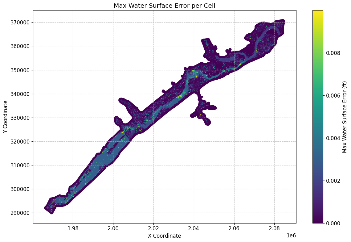
# Sort Dataframe to show top 10 maximum water surface errors:
max_ws_err_gdf_sorted = max_ws_err_gdf.sort_values(by='cell_maximum_water_surface_error', ascending=False)
Top 10 maximum water surface errors:
| mesh_name | cell_id | cell_maximum_water_surface_error | cell_maximum_water_surface_error_time | is_ghost_cell | geometry | x | y | |
|---|---|---|---|---|---|---|---|---|
| 17721 | BaldEagleCr | 17721 | 3.701377 | 2018-09-09 09:56:00 | False | POINT (2007386.39 321546.774) | 2.007386e+06 | 321546.773898 |
| 13520 | BaldEagleCr | 13520 | 1.786581 | 2018-09-09 10:13:20 | False | POINT (2007000 321250) | 2.007000e+06 | 321250.000000 |
| 13559 | BaldEagleCr | 13559 | 1.154887 | 2018-09-09 09:56:00 | False | POINT (2007000 321000) | 2.007000e+06 | 321000.000000 |
| 13558 | BaldEagleCr | 13558 | 0.076254 | 2018-09-09 09:56:00 | False | POINT (2006750 321000) | 2.006750e+06 | 321000.000000 |
| 13444 | BaldEagleCr | 13444 | 0.075218 | 2018-09-09 10:16:40 | False | POINT (2007500 321750) | 2.007500e+06 | 321750.000000 |
| ... | ... | ... | ... | ... | ... | ... | ... | ... |
| 770 | BaldEagleCr | 770 | 0.000007 | 2018-09-12 00:24:00 | False | POINT (2082500 366500) | 2.082500e+06 | 366500.000000 |
| 656 | BaldEagleCr | 656 | 0.000007 | 2018-09-12 01:23:40 | False | POINT (2082500 367000) | 2.082500e+06 | 367000.000000 |
| 657 | BaldEagleCr | 657 | 0.000007 | 2018-09-12 01:29:40 | False | POINT (2082750 367000) | 2.082750e+06 | 367000.000000 |
| 713 | BaldEagleCr | 713 | 0.000007 | 2018-09-12 01:45:00 | False | POINT (2082500 366750) | 2.082500e+06 | 366750.000000 |
| 658 | BaldEagleCr | 658 | 0.000006 | 2018-09-12 04:42:20 | False | POINT (2083000 367000) | 2.083000e+06 | 367000.000000 |
18066 rows × 8 columns
# Get mesh summary output for other Datasets (here we retrieve Maximum Face Courant) as geodataframe
max_courant_gdf = HdfResultsMesh.get_mesh_summary(plan_hdf_path, var="Maximum Face Courant")
Mesh Summary Output (Maximum Courant):


{'mesh_name': 'BaldEagleCr',
 'Can Interpolate': 'False',
 'Can Plot': 'True',
 'Coverage': 'Average',
 'Location': 'Faces',
 'Maximum Value of Data Set': np.float32(0.7945771),
 'Minimum Value of Data Set': np.float32(0.0),
 'Name': 'Face Courant Maximum',
 'Orientation': 'Scalar',
 'Row': np.int32(0),
 'Rows Variables': ['Courant Face', 'Time'],
 'Units': 'vel*dt/length',
 'Units per row': ['vel*dt/length', 'days']}
| mesh_name | face_id | maximum_face_courant | maximum_face_courant_time | geometry | |
|---|---|---|---|---|---|
| 0 | BaldEagleCr | 0 | 0.000017 | 2018-09-09 11:02:40 | LINESTRING (2042125 351625, 2042375 351625) |
| 1 | BaldEagleCr | 1 | 0.000062 | 2018-09-09 11:32:20 | LINESTRING (2042375 351625, 2042375 351875) |
| 2 | BaldEagleCr | 2 | 0.000038 | 2018-09-10 07:02:00 | LINESTRING (2042375 351875, 2042125 351875) |
| 3 | BaldEagleCr | 3 | 0.000016 | 2018-09-09 11:03:00 | LINESTRING (2042125 351875, 2042125 351625) |
| 4 | BaldEagleCr | 4 | 0.000056 | 2018-09-09 11:04:40 | LINESTRING (2042375 351375, 2042375 351625) |
| ... | ... | ... | ... | ... | ... |
| 37589 | BaldEagleCr | 37589 | 0.000000 | 2018-09-09 00:00:00 | LINESTRING (1978444.054 300812.794, 1978402.01... |
| 37590 | BaldEagleCr | 37590 | 0.000000 | 2018-09-09 00:00:00 | LINESTRING (1973531.76 297370.846, 1973246.989... |
| 37591 | BaldEagleCr | 37591 | 0.000000 | 2018-09-09 00:00:00 | LINESTRING (1968886.801 295900.5, 1968782.778 ... |
| 37592 | BaldEagleCr | 37592 | 0.000000 | 2018-09-09 00:00:00 | LINESTRING (1965981.775 291978.68, 1966280.11 ... |
| 37593 | BaldEagleCr | 37593 | 0.000000 | 2018-09-09 00:00:00 | LINESTRING (1969588.438 289578.114, 1969731.65... |
37594 rows × 5 columns
# Plot max Courant number

# Convert to GeoDataFrame if not empty
if not max_courant_gdf.empty:
    if generate_maps:
        # Get centroids of line geometries for plotting
        max_courant_gdf['centroid'] = max_courant_gdf.geometry.centroid
        max_courant_gdf['x'] = max_courant_gdf.centroid.x
        max_courant_gdf['y'] = max_courant_gdf.centroid.y

        # Create the plot
        fig, ax = plt.subplots(figsize=(12, 8))
        scatter = ax.scatter(max_courant_gdf['x'], max_courant_gdf['y'],
                        c=max_courant_gdf['maximum_face_courant'],
                        cmap='viridis',
                        s=10)

        # Customize the plot
        ax.set_title('Max Courant Number per Face')
        ax.set_xlabel('X Coordinate')
        ax.set_ylabel('Y Coordinate')
        plt.colorbar(scatter, label='Max Courant Number')

        # Add grid lines
        ax.grid(True, linestyle='--', alpha=0.7)

        # Increase font size for better readability
        plt.rcParams.update({'font.size': 12})

        # Adjust layout to prevent cutting off labels
        plt.tight_layout()

        # Show the plot
        plt.show()

# Print the first few rows of the dataframe for verification
print("\nFirst few rows of the Courant number dataframe:")
max_courant_gdf
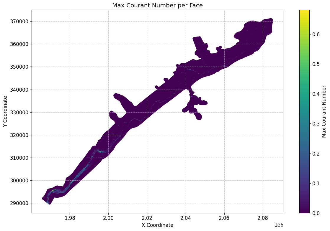
First few rows of the Courant number dataframe:
| mesh_name | face_id | maximum_face_courant | maximum_face_courant_time | geometry | centroid | x | y | |
|---|---|---|---|---|---|---|---|---|
| 0 | BaldEagleCr | 0 | 0.000017 | 2018-09-09 11:02:40 | LINESTRING (2042125 351625, 2042375 351625) | POINT (2042250 351625) | 2.042250e+06 | 351625.000000 |
| 1 | BaldEagleCr | 1 | 0.000062 | 2018-09-09 11:32:20 | LINESTRING (2042375 351625, 2042375 351875) | POINT (2042375 351750) | 2.042375e+06 | 351750.000000 |
| 2 | BaldEagleCr | 2 | 0.000038 | 2018-09-10 07:02:00 | LINESTRING (2042375 351875, 2042125 351875) | POINT (2042250 351875) | 2.042250e+06 | 351875.000000 |
| 3 | BaldEagleCr | 3 | 0.000016 | 2018-09-09 11:03:00 | LINESTRING (2042125 351875, 2042125 351625) | POINT (2042125 351750) | 2.042125e+06 | 351750.000000 |
| 4 | BaldEagleCr | 4 | 0.000056 | 2018-09-09 11:04:40 | LINESTRING (2042375 351375, 2042375 351625) | POINT (2042375 351500) | 2.042375e+06 | 351500.000000 |
| ... | ... | ... | ... | ... | ... | ... | ... | ... |
| 37589 | BaldEagleCr | 37589 | 0.000000 | 2018-09-09 00:00:00 | LINESTRING (1978444.054 300812.794, 1978402.01... | POINT (1978423.032 300718.897) | 1.978423e+06 | 300718.897016 |
| 37590 | BaldEagleCr | 37590 | 0.000000 | 2018-09-09 00:00:00 | LINESTRING (1973531.76 297370.846, 1973246.989... | POINT (1973389.375 297311.928) | 1.973389e+06 | 297311.928472 |
| 37591 | BaldEagleCr | 37591 | 0.000000 | 2018-09-09 00:00:00 | LINESTRING (1968886.801 295900.5, 1968782.778 ... | POINT (1968834.79 295808.861) | 1.968835e+06 | 295808.860743 |
| 37592 | BaldEagleCr | 37592 | 0.000000 | 2018-09-09 00:00:00 | LINESTRING (1965981.775 291978.68, 1966280.11 ... | POINT (1966130.942 291879.395) | 1.966131e+06 | 291879.394946 |
| 37593 | BaldEagleCr | 37593 | 0.000000 | 2018-09-09 00:00:00 | LINESTRING (1969588.438 289578.114, 1969731.65... | POINT (1969660.046 289673.23) | 1.969660e+06 | 289673.230118 |
37594 rows × 8 columns
# Get mesh summary output for other Datasets (here we retrieve Maximum Face Courant)

max_face_shear_gdf = HdfResultsMesh.get_mesh_summary(plan_hdf_path, var="Maximum Face Shear Stress")
Mesh Summary Output (Maximum Face Shear Stress:
{'mesh_name': 'BaldEagleCr', 'Max Time': np.float32(0.0), 'Max Value': np.float32(0.0), 'Min Time': np.float32(0.0), 'Min Value': np.float32(0.0), 'Rows Variables': ['Shear Stress', 'Time'], 'Units': ['PSF', 'days']}
| mesh_name | face_id | maximum_face_shear_stress | maximum_face_shear_stress_time | geometry | |
|---|---|---|---|---|---|
| 0 | BaldEagleCr | 0 | 0.0 | 2018-09-09 | LINESTRING (2042125 351625, 2042375 351625) |
| 1 | BaldEagleCr | 1 | 0.0 | 2018-09-09 | LINESTRING (2042375 351625, 2042375 351875) |
| 2 | BaldEagleCr | 2 | 0.0 | 2018-09-09 | LINESTRING (2042375 351875, 2042125 351875) |
| 3 | BaldEagleCr | 3 | 0.0 | 2018-09-09 | LINESTRING (2042125 351875, 2042125 351625) |
| 4 | BaldEagleCr | 4 | 0.0 | 2018-09-09 | LINESTRING (2042375 351375, 2042375 351625) |
| ... | ... | ... | ... | ... | ... |
| 37589 | BaldEagleCr | 37589 | 0.0 | 2018-09-09 | LINESTRING (1978444.054 300812.794, 1978402.01... |
| 37590 | BaldEagleCr | 37590 | 0.0 | 2018-09-09 | LINESTRING (1973531.76 297370.846, 1973246.989... |
| 37591 | BaldEagleCr | 37591 | 0.0 | 2018-09-09 | LINESTRING (1968886.801 295900.5, 1968782.778 ... |
| 37592 | BaldEagleCr | 37592 | 0.0 | 2018-09-09 | LINESTRING (1965981.775 291978.68, 1966280.11 ... |
| 37593 | BaldEagleCr | 37593 | 0.0 | 2018-09-09 | LINESTRING (1969588.438 289578.114, 1969731.65... |
37594 rows × 5 columns
# Plot max face shear stress

if generate_maps and not max_face_shear_gdf.empty:
    # Calculate centroids of the line geometries and extract coordinates
    max_face_shear_gdf['centroid'] = max_face_shear_gdf['geometry'].apply(lambda line: line.centroid)
    max_face_shear_gdf['x'] = max_face_shear_gdf['centroid'].apply(lambda point: point.x)
    max_face_shear_gdf['y'] = max_face_shear_gdf['centroid'].apply(lambda point: point.y)

    # Create the plot
    fig, ax = plt.subplots(figsize=(12, 8))
    scatter = ax.scatter(max_face_shear_gdf['x'], max_face_shear_gdf['y'],
                        c=max_face_shear_gdf['maximum_face_shear_stress'],
                        cmap='viridis',
                        s=10)

    # Customize the plot
    ax.set_title('Max Face Shear Stress per Face')
    ax.set_xlabel('X Coordinate')
    ax.set_ylabel('Y Coordinate')
    plt.colorbar(scatter, label='Max Face Shear Stress (PSF)')

    # Add grid lines
    ax.grid(True, linestyle='--', alpha=0.7)

    # Increase font size for better readability
    plt.rcParams.update({'font.size': 12})

    # Adjust layout to prevent cutting off labels
    plt.tight_layout()

    # Show the plot
    plt.show()
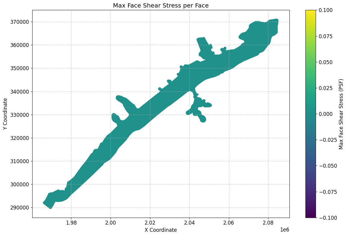
# Get mesh summary output for Minimum Water Surface as geodataframe
summary_gdf_min_ws = HdfResultsMesh.get_mesh_summary(plan_hdf_path, var="Minimum Water Surface")
Mesh Summary Output (Minimum Water Surface):
| mesh_name | cell_id | minimum_water_surface | minimum_water_surface_time | is_ghost_cell | geometry | |
|---|---|---|---|---|---|---|
| 0 | BaldEagleCr | 0 | 701.151245 | 2018-09-09 00:00:20 | False | POINT (2083000 370750) |
| 1 | BaldEagleCr | 1 | 689.052246 | 2018-09-09 00:00:20 | False | POINT (2083250 370750) |
| 2 | BaldEagleCr | 2 | 669.774719 | 2018-09-09 00:00:20 | False | POINT (2083500 370750) |
| 3 | BaldEagleCr | 3 | 658.986938 | 2018-09-09 00:00:20 | False | POINT (2083750 370750) |
| 4 | BaldEagleCr | 4 | 658.720581 | 2018-09-09 00:00:20 | False | POINT (2084000 370750) |
| ... | ... | ... | ... | ... | ... | ... |
| 18061 | BaldEagleCr | 18061 | 550.192688 | 2018-09-09 00:00:20 | False | POINT (2060527.525 351824.248) |
| 18062 | BaldEagleCr | 18062 | 550.218750 | 2018-09-09 00:00:20 | False | POINT (2060770.734 351834.938) |
| 18063 | BaldEagleCr | 18063 | 550.218750 | 2018-09-09 00:00:20 | False | POINT (2060928.42 351836.275) |
| 18064 | BaldEagleCr | 18064 | 567.500488 | 2018-09-09 00:00:20 | False | POINT (2061024.634 351710.661) |
| 18065 | BaldEagleCr | 18065 | 551.280029 | 2018-09-09 00:00:20 | False | POINT (2061115.504 351702.643) |
18066 rows × 6 columns
# Get mesh summary output for Minimum Face Velocity as geodataframe
summary_gdf_min_fv = HdfResultsMesh.get_mesh_summary(plan_hdf_path, var="Minimum Face Velocity")
Mesh Summary Output (Minimum Face Velocity):
| mesh_name | face_id | minimum_face_velocity | minimum_face_velocity_time | geometry | |
|---|---|---|---|---|---|
| 0 | BaldEagleCr | 0 | 0.0 | 2018-09-09 00:00:20 | LINESTRING (2042125 351625, 2042375 351625) |
| 1 | BaldEagleCr | 1 | 0.0 | 2018-09-09 00:00:20 | LINESTRING (2042375 351625, 2042375 351875) |
| 2 | BaldEagleCr | 2 | 0.0 | 2018-09-09 00:00:20 | LINESTRING (2042375 351875, 2042125 351875) |
| 3 | BaldEagleCr | 3 | 0.0 | 2018-09-09 00:00:20 | LINESTRING (2042125 351875, 2042125 351625) |
| 4 | BaldEagleCr | 4 | 0.0 | 2018-09-09 00:00:20 | LINESTRING (2042375 351375, 2042375 351625) |
| ... | ... | ... | ... | ... | ... |
| 37589 | BaldEagleCr | 37589 | 0.0 | 2018-09-09 00:00:20 | LINESTRING (1978444.054 300812.794, 1978402.01... |
| 37590 | BaldEagleCr | 37590 | 0.0 | 2018-09-09 00:00:20 | LINESTRING (1973531.76 297370.846, 1973246.989... |
| 37591 | BaldEagleCr | 37591 | 0.0 | 2018-09-09 00:00:20 | LINESTRING (1968886.801 295900.5, 1968782.778 ... |
| 37592 | BaldEagleCr | 37592 | 0.0 | 2018-09-09 00:00:20 | LINESTRING (1965981.775 291978.68, 1966280.11 ... |
| 37593 | BaldEagleCr | 37593 | 0.0 | 2018-09-09 00:00:20 | LINESTRING (1969588.438 289578.114, 1969731.65... |
37594 rows × 5 columns
# Get mesh summary output for Cell Cumulative Iteration as geodataframe
summary_gdf_cum_iter = HdfResultsMesh.get_mesh_summary(plan_hdf_path, var="Cell Cumulative Iteration")
Mesh Summary Output (Cell Cumulative Iteration):
| mesh_name | cell_id | cell_cumulative_iteration | is_ghost_cell | geometry | |
|---|---|---|---|---|---|
| 0 | BaldEagleCr | 0 | 0.0 | False | POINT (2083000 370750) |
| 1 | BaldEagleCr | 1 | 0.0 | False | POINT (2083250 370750) |
| 2 | BaldEagleCr | 2 | 0.0 | False | POINT (2083500 370750) |
| 3 | BaldEagleCr | 3 | 0.0 | False | POINT (2083750 370750) |
| 4 | BaldEagleCr | 4 | 0.0 | False | POINT (2084000 370750) |
| ... | ... | ... | ... | ... | ... |
| 18061 | BaldEagleCr | 18061 | 0.0 | False | POINT (2060527.525 351824.248) |
| 18062 | BaldEagleCr | 18062 | 0.0 | False | POINT (2060770.734 351834.938) |
| 18063 | BaldEagleCr | 18063 | 0.0 | False | POINT (2060928.42 351836.275) |
| 18064 | BaldEagleCr | 18064 | 0.0 | False | POINT (2061024.634 351710.661) |
| 18065 | BaldEagleCr | 18065 | 0.0 | False | POINT (2061115.504 351702.643) |
18066 rows × 5 columns
# Get mesh timeseries output as xarray
# The mesh name is part of the timeseries HDF path, so you must pass the mesh_name to retrieve it

# Get mesh areas from previous code cell
mesh_areas = HdfMesh.get_mesh_area_names(geom_hdf_path)
['BaldEagleCr']
# Use the first mesh area name to extract mesh timeseries output as xarray
timeseries_xr = HdfResultsMesh.get_mesh_timeseries(plan_hdf_path, mesh_areas[0], "Water Surface") # Use the first 2D flow area name for mesh_name
<xarray.DataArray (time: 721, cell_id: 18066)> Size: 52MB
array([[701.15125, 689.05225, 669.7747 , ..., 550.21875, 567.5003 ,
        551.2798 ],
       [701.15125, 689.05225, 669.7747 , ..., 550.21875, 567.5067 ,
        551.28625],
       [701.15125, 689.05225, 669.7747 , ..., 550.21875, 567.5131 ,
        551.29266],
       ...,
       [701.75244, 689.7832 , 670.0496 , ..., 550.40607, 567.6704 ,
        551.333  ],
       [701.7519 , 689.7825 , 670.0493 , ..., 550.40607, 567.6704 ,
        551.33295],
       [701.7513 , 689.7818 , 670.0491 , ..., 550.406  , 567.67035,
        551.3329 ]], shape=(721, 18066), dtype=float32)
Coordinates:
  * time           (time) datetime64[ns] 6kB 2018-09-09 ... 2018-09-14
  * cell_id        (cell_id) int64 145kB 0 1 2 3 4 ... 18062 18063 18064 18065
    is_ghost_cell  (cell_id) bool 18kB False False False ... False False False
Attributes:
    units:      ft
    mesh_name:  BaldEagleCr
variable: Water Surface# Time Series Output Variables for Cells
#
# Variable Name: Description
# Water Surface: Water surface elevation
# Depth: Water depth
# Velocity: Magnitude of velocity
# Velocity X: X-component of velocity
# Velocity Y: Y-component of velocity
# Froude Number: Froude number
# Courant Number: Courant number
# Shear Stress: Shear stress on the bed
# Bed Elevation: Elevation of the bed
# Precipitation Rate: Rate of precipitation
# Infiltration Rate: Rate of infiltration
# Evaporation Rate: Rate of evaporation
# Percolation Rate: Rate of percolation
# Groundwater Elevation: Elevation of groundwater
# Groundwater Depth: Depth to groundwater
# Groundwater Flow: Groundwater flow rate
# Groundwater Velocity: Magnitude of groundwater velocity
# Groundwater Velocity X: X-component of groundwater velocity
# Groundwater Velocity Y: Y-component of groundwater velocity
#
# These variables are available for time series output at the cell level in 2D flow areas.
# Get mesh cells water-surface timeseries output as xarray
cells_timeseries_xr = HdfResultsMesh.get_mesh_cells_timeseries(
    plan_hdf_path,
    mesh_areas[0],
    var="Water Surface",
)
{'BaldEagleCr': <xarray.Dataset> Size: 52MB
 Dimensions:        (time: 721, cell_id: 18066)
 Coordinates:
   * time           (time) datetime64[us] 6kB 2018-09-09 ... 2018-09-14
   * cell_id        (cell_id) int64 145kB 0 1 2 3 4 ... 18062 18063 18064 18065
     is_ghost_cell  (cell_id) bool 18kB False False False ... False False False
 Data variables:
     Water Surface  (time, cell_id) float32 52MB 701.2 689.1 ... 567.7 551.3
 Attributes:
     mesh_name:   BaldEagleCr
     start_time:  2018-09-09 00:00:00}
# Plot WSE Time Series Data (Random Cell ID)
import matplotlib.pyplot as plt

if generate_plots:
    import numpy as np
    import random

    # Extract Water Surface data
    water_surface = cells_timeseries_xr[mesh_areas[0]]['Water Surface']

    # Get the time values
    time_values = water_surface.coords['time'].values

    # Pick a random cell_id
    random_cell_id = random.choice(water_surface.coords['cell_id'].values)

    # Extract the water surface elevation time series for the random cell
    wsel_timeseries = water_surface.sel(cell_id=random_cell_id)

    # Find the peak value and its index
    peak_value = wsel_timeseries.max().item()
    peak_index = wsel_timeseries.argmax().item()

    # Create the plot
    plt.figure(figsize=(12, 6))
    plt.plot(time_values, wsel_timeseries, label=f'Cell ID: {random_cell_id}')
    plt.scatter(time_values[peak_index], peak_value, color='red', s=100, zorder=5)
    plt.annotate(f'Peak: {peak_value:.2f} ft',
                (time_values[peak_index], peak_value),
                xytext=(10, 10), textcoords='offset points',
                ha='left', va='bottom',
                bbox=dict(boxstyle='round,pad=0.5', fc='yellow', alpha=0.5),
                arrowprops=dict(arrowstyle='->', connectionstyle='arc3,rad=0'))

    plt.title(f'Water Surface Elevation Time Series for Random Cell (ID: {random_cell_id})')
    plt.xlabel('Time')
    plt.ylabel('Water Surface Elevation (ft)')
    plt.legend()
    plt.grid(True)
    plt.tight_layout()

    # Log the plotting action
    logging.info(f"Plotted water surface elevation time series for random cell ID: {random_cell_id}")

    # Display the plot
    plt.show()

    # Print some statistics
    print(f"Statistics for Cell ID {random_cell_id}:")
    print(f"Minimum WSEL: {wsel_timeseries.min().item():.2f} ft")
    print(f"Maximum WSEL: {peak_value:.2f} ft")
    print(f"Mean WSEL: {wsel_timeseries.mean().item():.2f} ft")
    print(f"Time of peak: {time_values[peak_index]}")
D:\CLB-Temp\clb-t3-pr534\venv2\Lib\site-packages\xarray\core\dataarray.py:6563: FutureWarning: Behaviour of argmin/argmax with neither dim nor axis argument will change to return a dict of indices of each dimension. To get a single, flat index, please use np.argmin(da.data) or np.argmax(da.data) instead of da.argmin() or da.argmax().
  result = self.variable.argmax(dim, axis, keep_attrs, skipna)
2026-10-15 15:40:19 - root - INFO - Plotted water surface elevation time series for random cell ID: 5903
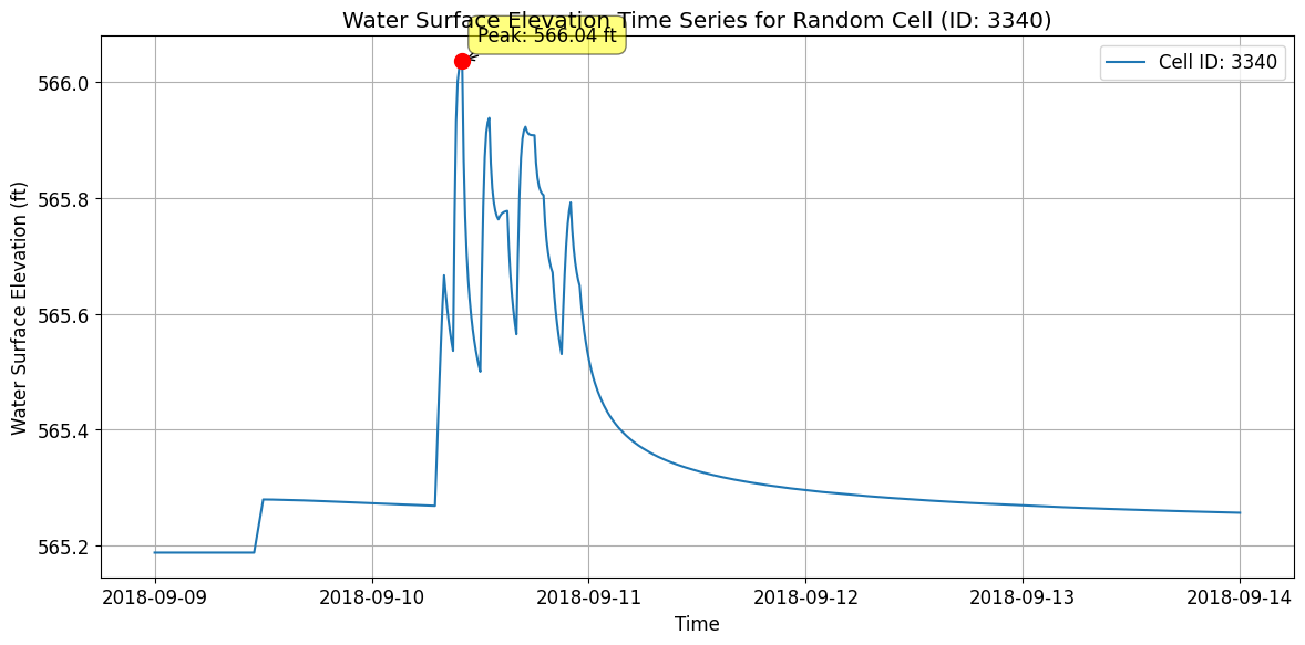
Statistics for Cell ID 5903:
Minimum WSEL: 569.55 ft
Maximum WSEL: 570.73 ft
Mean WSEL: 569.98 ft
Time of peak: 2018-09-10T18:00:00.000000
# Get mesh faces timeseries output as xarray
faces_timeseries_xr = HdfResultsMesh.get_mesh_faces_timeseries(plan_hdf_path, mesh_areas[0])
<xarray.Dataset> Size: 542MB
Dimensions:              (time: 721, face_id: 37594)
Coordinates:
  * time                 (time) datetime64[ns] 6kB 2018-09-09 ... 2018-09-14
  * face_id              (face_id) int64 301kB 0 1 2 3 ... 37591 37592 37593
Data variables:
    face_flow            (time, face_id) float32 108MB nan nan nan ... 0.0 0.0
    face_velocity        (time, face_id) float32 108MB nan nan nan ... 0.0 0.0
    face_water_surface   (time, face_id) float32 108MB 620.1 630.9 ... 782.4
    face_eddy_viscosity  (time, face_id) float32 108MB 0.0 0.0 0.0 ... 0.0 0.0
    face_shear_stress    (time, face_id) float32 108MB nan nan nan ... 0.0 0.0
Attributes:
    units:      cfs
    mesh_name:  BaldEagleCr
variable: Face Flow# Plot Random Face Results and Label Peak, Plus Map View
if generate_maps:
# Select a random valid face ID number
random_face = np.random.randint(0, faces_timeseries_xr.sizes['face_id'])
# Extract time series data for the selected face
variable = 'face_velocity' # We could also use 'face_flow'
face_data = faces_timeseries_xr[variable].sel(face_id=random_face)
# Find peak value and its corresponding time
peak_value = face_data.max().item()
peak_time = face_data.idxmax().values
# Plot time series
plt.figure(figsize=(12, 8))
plt.plot(faces_timeseries_xr.time, face_data)
plt.title(f'{variable.capitalize()} Time Series for Face {random_face}')
plt.xlabel('Time')
plt.ylabel(f'{variable.capitalize()} ({faces_timeseries_xr.attrs["units"]})')
plt.grid(True)
# Annotate the peak point
plt.annotate(f'Peak: ({peak_time}, {peak_value:.2f})',
(peak_time, peak_value),
xytext=(10, 10), textcoords='offset points',
arrowprops=dict(arrowstyle="->"))
# Check for negative values and label the minimum if present
min_value = face_data.min().item()
if min_value < 0:
min_time = face_data.idxmin().values
plt.annotate(f'Min: ({min_time}, {min_value:.2f})',
(min_time, min_value),
xytext=(10, -10), textcoords='offset points',
arrowprops=dict(arrowstyle="->"))
plt.tight_layout()
plt.show()
# Create map view plot
fig, ax = plt.subplots(figsize=(12, 8))
# Calculate mesh faces extents with 10% buffer
faces_bounds = mesh_cell_faces_gdf.total_bounds
x_min, y_min, x_max, y_max = faces_bounds
buffer_x = (x_max - x_min) * 0.1
buffer_y = (y_max - y_min) * 0.1
plot_xlim = [x_min - buffer_x, x_max + buffer_x]
plot_ylim = [y_min - buffer_y, y_max + buffer_y]
# Set plot limits before adding terrain
ax.set_xlim(plot_xlim)
ax.set_ylim(plot_ylim)
# Add the terrain TIFF to the map if available
tiff_path = Path.cwd() / 'example_projects' / 'BaldEagleCrkMulti2D' / 'Terrain' / 'Terrain50.baldeagledem.tif'
if tiff_path.exists():
with rasterio.open(tiff_path) as src:
show(src, ax=ax, cmap='terrain', alpha=0.5)
else:
logging.info(f'Terrain TIFF not found at {tiff_path}, skipping terrain overlay')
# Reset the limits after terrain plot
ax.set_xlim(plot_xlim)
ax.set_ylim(plot_ylim)
# Plot all faces in gray
mesh_cell_faces_gdf.plot(ax=ax, color='lightgray', alpha=0.5, zorder=2)
# Get the selected face geometry
selected_face = mesh_cell_faces_gdf[mesh_cell_faces_gdf['face_id'] == random_face]
# Highlight the selected face in red
selected_face.plot(
ax=ax,
color='red',
linewidth=2,
label=f'Selected Face (ID: {random_face})',
zorder=3
)
# Get bounds of selected face for zoomed inset
bounds = selected_face.geometry.bounds.iloc[0]
x_center = (bounds.iloc[0] + bounds.iloc[2]) / 2
y_center = (bounds.iloc[1] + bounds.iloc[3]) / 2
buffer = max(bounds.iloc[2] - bounds.iloc[0], bounds.iloc[3] - bounds.iloc[1]) * 2
# Create zoomed inset with a larger size, inside the map frame
axins = inset_axes(ax, width="70%", height="70%", loc='lower right',
bbox_to_anchor=(0.65, 0.05, 0.35, 0.35),
bbox_transform=ax.transAxes)
# Plot terrain and faces in inset (if available)
if tiff_path.exists():
with rasterio.open(tiff_path) as src:
show(src, ax=axins, cmap='terrain', alpha=0.5)
# Plot zoomed view in inset
mesh_cell_faces_gdf.plot(ax=axins, color='lightgray', alpha=0.5, zorder=2)
selected_face.plot(ax=axins, color='red', linewidth=2, zorder=3)
# Set inset limits with slightly more context
axins.set_xlim(x_center - buffer/1.5, x_center + buffer/1.5)
axins.set_ylim(y_center - buffer/1.5, y_center + buffer/1.5)
# Remove inset ticks for cleaner look
axins.set_xticks([])
axins.set_yticks([])
# Add a border to the inset
for spine in axins.spines.values():
spine.set_edgecolor('black')
spine.set_linewidth(1.5)
# Create connection lines between main plot and inset
# Get the selected face centroid for connection point
centroid = selected_face.geometry.centroid.iloc[0]
con1 = ConnectionPatch(
xyA=(centroid.x, centroid.y), coordsA=ax.transData,
xyB=(0.02, 0.98), coordsB=axins.transAxes,
arrowstyle="-", linestyle="--", color="gray", alpha=0.6
)
con2 = ConnectionPatch(
xyA=(centroid.x, centroid.y), coordsA=ax.transData,
xyB=(0.98, 0.02), coordsB=axins.transAxes,
arrowstyle="-", linestyle="--", color="gray", alpha=0.6
)
ax.add_artist(con1)
ax.add_artist(con2)
# Add title and legend to main plot
ax.set_title('Mesh Face Map View with Terrain')
ax.legend()
# Ensure equal aspect ratio while maintaining our desired extents
ax.set_aspect('equal', adjustable='box')
plt.tight_layout()
plt.show()
# Print summary information
print(f"Random Face: {random_face}")
print(f"Peak Value: {peak_value:.2f} {faces_timeseries_xr.attrs['units']} at {peak_time}")
if min_value < 0:
print(f"Minimum Value: {min_value:.2f} {faces_timeseries_xr.attrs['units']} at {min_time}")
# Log the plotting action
logging.info(f"Plotted mesh face time series and map view for random face ID: {random_face} with terrain")
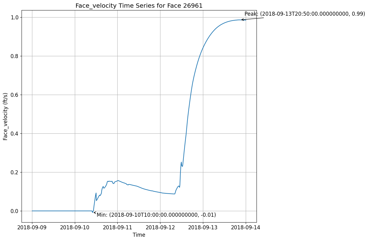
2026-10-15 15:40:22 - root - INFO - Terrain TIFF not found at D:\CLB-Temp\clb-t3-pr534\repo2\examples\example_projects\BaldEagleCrkMulti2D\Terrain\Terrain50.baldeagledem.tif, skipping terrain overlay


C:\Users\billk_clb\AppData\Local\Temp\ipykernel_19768\423459082.py:142: UserWarning: This figure includes Axes that are not compatible with tight_layout, so results might be incorrect.
  plt.tight_layout()
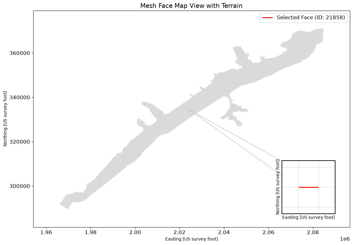
2026-10-15 15:40:24 - root - INFO - Plotted mesh face time series and map view for random face ID: 21858 with terrain


Random Face: 21858
Peak Value: 0.04 cfs at 2018-09-09T15:00:00.000000000
Minimum Value: -0.53 cfs at 2018-09-12T20:10:00.000000000
# Get meteorology precipitation attributes
meteo_precip_attrs = HdfPlan.get_plan_met_precip(plan_hdf_path)
{'DSS Filename': '.\\Precipitation\\precip.2018.09.dss',
 'DSS Pathname': '/SHG/MARFC/PRECIP/01SEP2018:0200/01SEP2018:0300/NEXRAD/',
 'Data Type': 'per-cum',
 'Interpolation Method': '',
 'Mode': 'Gridded',
 'Projection': 'PROJCS["USA_Contiguous_Albers_Equal_Area_Conic_USGS_version",GEOGCS["NAD83",DATUM["North_American_Datum_1983",SPHEROID["GRS 1980",6378137,298.257222101,AUTHORITY["EPSG","7019"]],AUTHORITY["EPSG","6269"]],PRIMEM["Greenwich",0],UNIT["Degree",0.0174532925199433]],PROJECTION["Albers_Conic_Equal_Area"],PARAMETER["latitude_of_center",23],PARAMETER["longitude_of_center",-96],PARAMETER["standard_parallel_1",29.5],PARAMETER["standard_parallel_2",45.5],PARAMETER["false_easting",0],PARAMETER["false_northing",0],UNIT["metre",1,AUTHORITY["EPSG","9001"]],AXIS["Easting",EAST],AXIS["Northing",NORTH]]',
 'Raster Cellsize': np.float64(2000.0),
 'Raster Cols': np.int32(515),
 'Raster Left': np.float64(1096000.0),
 'Raster Rows': np.int32(522),
 'Raster Top': np.float64(2560000.0),
 'Source': 'DSS',
 'Units': 'in'}
# Get results unsteady attributes
results_unsteady_attrs = HdfResultsPlan.get_unsteady_info(plan_hdf_path)
| Plan Title | Program Name | Program Version | Project File Name | Project Title | Short ID | Simulation Time Window | Type of Run | |
|---|---|---|---|---|---|---|---|---|
| 0 | Gridded Precip - Infiltration | HEC-RAS - River Analysis System | HEC-RAS 7.0 April 2026 | D:\CLB-Temp\clb-t3-pr534\repo2\examples\exampl... | Bald Eagle Creek Example Dam Break Study | Grid Precip Infiltration | 08Sep2018 2400 to 13Sep2018 2400 | Unsteady Flow Analysis |
# Get results unsteady summary attributes
results_unsteady_summary_attrs = HdfResultsPlan.get_unsteady_summary(plan_hdf_path)
| Computation Time DSS | Computation Time Total | Maximum WSEL Error | Maximum number of cores | Run Time Window | Solution | Time Solution Went Unstable | Time Stamp Solution Went Unstable | |
|---|---|---|---|---|---|---|---|---|
| 0 | 00:00:00 | 00:05:33 | 0.0 | 2 | 15OCT2026 03:48:39 to 15OCT2026 03:54:12 | Unsteady Finished Successfully | NaN | Not Applicable |
# Get results volume accounting attributes
volume_accounting_attrs = HdfResultsPlan.get_volume_accounting(plan_hdf_path)
| Error | Error Percent | Precipitation Excess (acre feet) | Precipitation Excess (inches) | Total Boundary Flux of Water In | Total Boundary Flux of Water Out | Vol Accounting in | Volume Ending | Volume Starting | |
|---|---|---|---|---|---|---|---|---|---|
| 0 | 0.610979 | 0.000431 | 3756.872803 | 1.707615 | 141685.265625 | 17253.21875 | Acre Feet | 124432.664062 | 0.0 |
# Extract Compute Messages as String
print("Extracting Compute Messages")

import h5py
import numpy as np


def extract_string_from_hdf(results_hdf_filename: str, hdf_path: str) -> str:
    """
    Extract string from HDF object at a given path

    Parameters
    ----------
    results_hdf_filename : str
        Name of the HDF file
    hdf_path : str
        Path of the object in the HDF file

    Returns
    -------
    str
        Extracted string from the specified HDF object
    """
    with h5py.File(results_hdf_filename, 'r') as hdf_file:
        try:
            hdf_object = hdf_file[hdf_path]
            if isinstance(hdf_object, h5py.Group):
                return f"Group: {hdf_path}\nContents: {list(hdf_object.keys())}"
            elif isinstance(hdf_object, h5py.Dataset):
                data = hdf_object[()]
                if isinstance(data, bytes):
                    return data.decode('utf-8')
                elif isinstance(data, np.ndarray) and data.dtype.kind == 'S':
                    return [v.decode('utf-8') for v in data]
                else:
                    return str(data)
            else:
                return f"Unsupported object type: {type(hdf_object)}"
        except KeyError:
            return f"Path not found: {hdf_path}"


try:
    results_summary_string = extract_string_from_hdf(plan_hdf_path, '/Results/Summary/Compute Messages (text)')
    print("Compute Messages:")

    # Parse and print the compute messages in a more visually friendly way
    messages = results_summary_string[0].split('\r\n')

    for message in messages:
        if message.strip():  # Skip empty lines
            if ':' in message:
                key, value = message.split(':', 1)
                print(f"{key.strip():40} : {value.strip()}")
            else:
                print(f"\n{message.strip()}")

    # Print computation summary in a table format
    print("\nComputation Summary:")
    print("-" * 50)
    print(f"{'Computation Task':<30} {'Time':<20}")
    print("-" * 50)
    for line in messages:
        if 'Computation Task' in line:
            task, time = line.split('\t')
            print(f"{task:<30} {time:<20}")

    print("\nComputation Speed:")
    print("-" * 50)
    print(f"{'Task':<30} {'Simulation/Runtime':<20}")
    print("-" * 50)
    for line in messages:
        if 'Computation Speed' in line:
            task, speed = line.split('\t')
            print(f"{task:<30} {speed:<20}")

except Exception as e:
    print(f"Error extracting compute messages: {str(e)}")
    print("\nNote: If 'Results/Summary Output' is not in the file structure, it might indicate that the simulation didn't complete successfully or the results weren't saved properly.")
Extracting Compute Messages
Compute Messages:
Plan : 'Gridded Precip - Infiltration' (BaldEagleDamBrk.p06)
Simulation started at : 15Oct2026 03:48:26 AM
Writing Plan GIS Data...
Completed Writing Plan GIS Data
Writing Geometry...
Terrain : Terrain50
Land Cover : LandCover
Infiltration : Infiltration
Percent Impervious : LandCover
Computing 2D Flow Area 'BaldEagleCr' tables : Property tables do not exist.
2D Flow Area 'BaldEagleCr' tables complete 8.61 sec
Completed Writing Geometry
Writing Event Conditions ...
Processing Precipitation data...
(assumes geometry data is geo-referenced)
Finished Processing Precipitation data (1.41s)
Completed Writing Event Condition Data
Geometric Preprocessor HEC-RAS 7.0 April 2026
Finished Processing Geometry
Parallelization CPU Affinity ON (Performance Cores 0,1)
Performing Unsteady Flow Simulation HEC-RAS 7.0 April 2026
Unsteady Input Summary :
2D Area Cells Cores Solvers
BaldEagleCr 18066 2 Diffusion Wave Equation Set (fastest)
Maximum adaptive timestep = 40.0 Minimum adaptive timestep = 20.0
Initial adaptive timestep = 20.0
09SEP2018 00 : 01:20 timestep = 40 (sec)
Maximum iteration location Cell WSEL ERROR ITERATIONS
09SEP2018 02 : 50:00 BaldEagleCr 17721 585.43 0.052 20
09SEP2018 03 : 42:40 BaldEagleCr 17721 585.62 0.012 20
09SEP2018 04 : 27:20 BaldEagleCr 17721 585.80 0.012 20
09SEP2018 05 : 09:20 BaldEagleCr 17721 585.97 0.012 20
09SEP2018 05 : 50:40 BaldEagleCr 17721 586.15 0.052 20
09SEP2018 06 : 38:00 BaldEagleCr 17721 586.33 0.052 20
09SEP2018 07 : 28:40 BaldEagleCr 17721 586.50 0.052 20
09SEP2018 08 : 23:20 BaldEagleCr 17721 586.67 0.052 20
09SEP2018 09 : 20:00 BaldEagleCr 17721 586.84 0.051 20
09SEP2018 09 : 34:40 BaldEagleCr 17721 586.95 0.051 20
09SEP2018 09 : 40:00 BaldEagleCr 17721 587.04 0.052 20
09SEP2018 09 : 43:20 BaldEagleCr 13559 595.06 0.312 20
09SEP2018 09 : 46:00 BaldEagleCr 13559 595.70 0.235 20
09SEP2018 09 : 48:00 BaldEagleCr 13559 596.06 0.216 20
09SEP2018 09 : 49:20 BaldEagleCr 13559 596.05 0.207 20
09SEP2018 09 : 50:40 BaldEagleCr 13559 596.47 0.160 20
09SEP2018 09 : 52:00 BaldEagleCr 17721 590.60 2.913 21
09SEP2018 09 : 53:20 BaldEagleCr 17721 590.22 3.114 20
09SEP2018 09 : 54:40 BaldEagleCr 17721 590.33 0.286 21
09SEP2018 09 : 56:00 BaldEagleCr 17721 591.51 3.701 21
09SEP2018 09 : 57:20 BaldEagleCr 17721 590.05 3.099 20
09SEP2018 09 : 58:40 BaldEagleCr 17721 591.18 0.542 21
09SEP2018 10 : 00:00 BaldEagleCr 17721 590.91 0.582 21
09SEP2018 10 : 01:20 BaldEagleCr 17721 591.03 0.562 20
09SEP2018 10 : 02:40 BaldEagleCr 17721 591.02 0.564 20
09SEP2018 10 : 04:00 BaldEagleCr 13520 592.66 0.624 21
09SEP2018 10 : 04:40 BaldEagleCr 17721 589.65 1.797 20
09SEP2018 10 : 05:20 BaldEagleCr 17721 590.48 0.681 21
09SEP2018 10 : 06:00 BaldEagleCr 13520 593.12 0.652 20
09SEP2018 10 : 06:40 BaldEagleCr 17721 592.01 1.366 20
09SEP2018 10 : 08:00 BaldEagleCr 13520 592.82 0.784 20
09SEP2018 10 : 08:40 BaldEagleCr 17721 587.80 0.407 20
09SEP2018 10 : 09:20 BaldEagleCr 13520 593.04 1.001 22
09SEP2018 10 : 10:00 BaldEagleCr 17721 589.02 1.222 20
09SEP2018 10 : 10:40 BaldEagleCr 17721 591.48 0.516 20
09SEP2018 10 : 12:00 BaldEagleCr 13520 592.78 0.741 21
09SEP2018 10 : 12:40 BaldEagleCr 13520 592.73 0.696 21
09SEP2018 10 : 13:20 BaldEagleCr 17721 592.17 1.291 21
09SEP2018 10 : 14:40 BaldEagleCr 13520 592.93 0.896 20
09SEP2018 10 : 15:20 BaldEagleCr 13520 592.87 0.836 21
09SEP2018 10 : 16:00 BaldEagleCr 13520 593.43 1.185 20
09SEP2018 10 : 16:40 BaldEagleCr 17721 588.00 0.663 20
09SEP2018 10 : 17:20 BaldEagleCr 17721 592.29 1.207 20
09SEP2018 10 : 18:40 BaldEagleCr 13520 592.17 1.342 21
09SEP2018 10 : 18:40 timestep = 20 (sec)
09SEP2018 10 : 19:20 BaldEagleCr 13520 593.80 0.925 21
09SEP2018 10 : 19:40 BaldEagleCr 13520 593.05 0.348 20
09SEP2018 10 : 20:00 BaldEagleCr 13520 593.80 0.850 21
09SEP2018 10 : 20:20 BaldEagleCr 13520 592.38 1.752 21
09SEP2018 10 : 20:40 BaldEagleCr 13520 592.53 0.308 20
09SEP2018 10 : 21:00 BaldEagleCr 17721 591.26 0.891 21
09SEP2018 10 : 21:20 BaldEagleCr 13520 593.13 0.308 20
09SEP2018 10 : 21:40 BaldEagleCr 13520 592.06 1.056 20
09SEP2018 10 : 22:20 BaldEagleCr 13520 593.32 0.417 20
09SEP2018 10 : 22:40 BaldEagleCr 13520 592.30 0.264 21
09SEP2018 10 : 23:00 BaldEagleCr 13520 593.24 0.312 20
09SEP2018 10 : 23:20 BaldEagleCr 13520 593.55 0.798 20
09SEP2018 10 : 23:40 BaldEagleCr 13520 593.40 0.437 20
09SEP2018 10 : 24:00 BaldEagleCr 13520 593.49 0.942 20
09SEP2018 10 : 24:20 BaldEagleCr 13520 593.38 0.437 20
09SEP2018 10 : 24:40 BaldEagleCr 13520 592.93 0.353 20
09SEP2018 10 : 25:00 BaldEagleCr 13520 592.47 0.431 21
09SEP2018 10 : 25:20 BaldEagleCr 13520 593.29 0.744 20
09SEP2018 10 : 25:40 BaldEagleCr 13520 593.68 0.970 21
09SEP2018 10 : 26:00 BaldEagleCr 13520 593.06 0.969 20
09SEP2018 10 : 26:20 BaldEagleCr 13520 593.14 1.045 21
09SEP2018 10 : 26:40 BaldEagleCr 13520 593.56 0.896 20
09SEP2018 10 : 27:00 BaldEagleCr 13520 593.35 0.479 20
09SEP2018 10 : 27:20 BaldEagleCr 13520 592.66 0.945 20
09SEP2018 10 : 27:40 BaldEagleCr 13520 592.19 1.206 20
09SEP2018 10 : 28:00 BaldEagleCr 13520 593.28 0.495 20
09SEP2018 10 : 28:20 BaldEagleCr 13520 593.27 0.515 20
09SEP2018 10 : 28:40 BaldEagleCr 13520 592.55 0.369 20
09SEP2018 10 : 29:00 BaldEagleCr 13520 592.86 0.459 20
09SEP2018 10 : 29:20 BaldEagleCr 13520 592.45 1.136 20
09SEP2018 10 : 29:40 BaldEagleCr 13520 592.89 0.454 20
09SEP2018 10 : 30:00 BaldEagleCr 13520 592.51 1.129 20
09SEP2018 10 : 30:20 BaldEagleCr 13520 593.24 0.446 20
09SEP2018 10 : 30:40 BaldEagleCr 13520 592.55 0.956 20
09SEP2018 10 : 31:00 BaldEagleCr 13520 593.39 0.408 20
09SEP2018 10 : 31:20 BaldEagleCr 13520 593.23 0.361 20
09SEP2018 10 : 31:40 BaldEagleCr 13520 592.69 0.315 20
09SEP2018 10 : 32:00 BaldEagleCr 13520 593.62 0.735 20
09SEP2018 10 : 32:20 BaldEagleCr 13520 593.15 0.181 20
09SEP2018 10 : 32:40 BaldEagleCr 13520 593.25 0.798 20
09SEP2018 10 : 33:00 BaldEagleCr 13520 592.98 0.155 20
09SEP2018 10 : 33:20 BaldEagleCr 13520 592.23 0.192 21
09SEP2018 10 : 33:40 BaldEagleCr 13520 593.45 0.461 20
09SEP2018 10 : 34:00 BaldEagleCr 13520 592.57 0.976 20
09SEP2018 10 : 34:20 BaldEagleCr 13520 593.28 0.496 20
09SEP2018 10 : 34:40 BaldEagleCr 13520 592.92 0.964 20
09SEP2018 10 : 35:00 BaldEagleCr 13520 592.86 0.240 20
09SEP2018 10 : 35:20 BaldEagleCr 13520 593.42 0.739 20
09SEP2018 10 : 35:40 BaldEagleCr 13520 593.26 0.139 20
09SEP2018 10 : 36:00 BaldEagleCr 13520 592.65 0.367 20
09SEP2018 10 : 36:20 BaldEagleCr 13520 593.25 0.244 20
09SEP2018 10 : 36:40 BaldEagleCr 13520 592.72 0.384 20
09SEP2018 10 : 37:00 BaldEagleCr 13520 593.25 0.246 20
09SEP2018 10 : 37:20 BaldEagleCr 13520 593.17 0.327 20
09SEP2018 10 : 37:40 BaldEagleCr 13520 592.95 0.101 20
09SEP2018 10 : 38:00 BaldEagleCr 13520 593.37 0.757 20
09SEP2018 10 : 38:20 BaldEagleCr 13520 593.11 0.017 20
09SEP2018 10 : 38:40 BaldEagleCr 13520 592.29 0.259 21
09SEP2018 10 : 39:00 BaldEagleCr 13520 593.01 0.114 20
09SEP2018 10 : 39:20 BaldEagleCr 13520 592.76 0.283 20
09SEP2018 10 : 39:40 BaldEagleCr 13520 593.29 0.077 20
09SEP2018 10 : 40:00 BaldEagleCr 13520 592.61 0.373 20
09SEP2018 10 : 40:20 BaldEagleCr 13520 593.18 0.084 20
09SEP2018 10 : 40:40 BaldEagleCr 13520 592.64 0.367 20
09SEP2018 10 : 41:00 BaldEagleCr 13520 593.24 0.084 20
09SEP2018 10 : 41:20 BaldEagleCr 13520 593.65 0.814 20
09SEP2018 10 : 42:00 BaldEagleCr 13520 593.12 0.990 20
09SEP2018 10 : 42:40 BaldEagleCr 13520 593.63 0.812 20
09SEP2018 10 : 43:20 BaldEagleCr 13520 592.59 0.767 20
09SEP2018 10 : 43:40 BaldEagleCr 13520 593.01 0.060 20
09SEP2018 10 : 44:00 BaldEagleCr 13520 592.69 0.935 20
09SEP2018 10 : 44:40 BaldEagleCr 13520 592.74 0.380 20
09SEP2018 10 : 45:20 BaldEagleCr 13520 593.02 0.973 20
09SEP2018 10 : 46:00 BaldEagleCr 13520 592.58 0.750 20
09SEP2018 10 : 46:40 BaldEagleCr 13520 593.05 0.944 20
09SEP2018 10 : 47:20 BaldEagleCr 13520 593.28 0.787 20
09SEP2018 10 : 48:00 BaldEagleCr 13520 592.58 0.543 20
09SEP2018 10 : 48:20 BaldEagleCr 13520 593.01 0.013 20
09SEP2018 10 : 48:40 BaldEagleCr 13520 594.15 1.303 20
09SEP2018 10 : 49:20 BaldEagleCr 13520 592.88 0.193 20
09SEP2018 10 : 49:40 BaldEagleCr 13520 592.97 0.136 20
09SEP2018 10 : 50:00 BaldEagleCr 13520 593.46 0.500 20
09SEP2018 10 : 50:40 BaldEagleCr 13520 592.66 0.366 20
09SEP2018 10 : 51:00 BaldEagleCr 13520 593.56 0.580 20
09SEP2018 10 : 51:20 BaldEagleCr 13520 593.51 0.285 20
09SEP2018 10 : 51:40 BaldEagleCr 13520 593.09 0.010 20
09SEP2018 10 : 52:00 BaldEagleCr 13520 593.33 0.541 20
09SEP2018 10 : 52:40 BaldEagleCr 13520 593.37 0.558 20
09SEP2018 10 : 53:20 BaldEagleCr 13520 592.80 0.207 20
09SEP2018 10 : 53:40 BaldEagleCr 13520 593.01 0.051 20
09SEP2018 10 : 54:00 BaldEagleCr 13520 593.48 0.546 21
09SEP2018 10 : 54:40 BaldEagleCr 13520 593.29 0.213 20
09SEP2018 10 : 55:20 BaldEagleCr 13520 593.54 0.579 20
09SEP2018 10 : 56:00 BaldEagleCr 13520 593.52 0.176 20
09SEP2018 10 : 56:40 BaldEagleCr 13520 593.56 0.174 20
09SEP2018 10 : 57:20 BaldEagleCr 13520 593.51 0.122 20
09SEP2018 10 : 58:00 BaldEagleCr 13520 593.04 0.012 20
09SEP2018 10 : 58:20 BaldEagleCr 13520 593.31 0.084 20
09SEP2018 10 : 59:40 BaldEagleCr 13520 593.62 0.624 20
09SEP2018 11 : 00:40 BaldEagleCr 13520 593.25 0.105 20
09SEP2018 11 : 01:20 BaldEagleCr 13520 592.95 0.092 20
09SEP2018 11 : 01:40 BaldEagleCr 13520 593.08 0.028 20
09SEP2018 11 : 02:00 BaldEagleCr 13520 593.21 0.105 20
09SEP2018 11 : 02:40 BaldEagleCr 13520 593.33 0.088 20
Overall Volume Accounting Error in Acre Feet : 0.6110
Overall Volume Accounting Error as percentage : 0.000431
Please review "Computational Log File" output for volume accounting details
Writing Results to DSS
The maximum cell wsel error was 3.70
At BaldEagleCr cell 17721
Finished Unsteady Flow Simulation
1D Post Process Skipped (simulation is all 2D)
Computations Summary
Computation Task Time(hh : mm:ss)
Completing Geometry, Flow and Plan 12
Preprocessing Geometry <1
Unsteady Flow Computations 5 : 34
Complete Process 5 : 46
Computation Speed Simulation/Runtime
Unsteady Flow Computations 1292x
Complete Process 1246x
Computation Summary:
--------------------------------------------------
Computation Task Time
--------------------------------------------------
Computation Task Time(hh:mm:ss)
Computation Speed:
--------------------------------------------------
Task Simulation/Runtime
--------------------------------------------------
Computation Speed Simulation/Runtime
Exploring HDF Datasets with HdfBase.get_dataset_info
This allows users to find HDF information that is not included in the ras-commander library. Find the path in HDFView and set the group_path below to explore the HDF datasets and attributes. Then, use the output to write your own function to extract the data.
Get HDF Paths with Properties (For Exploring HDF Files)
HdfBase.get_dataset_info(plan_number, group_path="/")
Common 2D Mesh Extraction Patterns
Pattern 1: Extract Maximum Inundation
# READ maximum depth from an existing HEC-RAS result HDF.
# Stored Depth is used when present; otherwise ras-commander DERIVES values
# in memory from Water Surface minus Cells Minimum Elevation. It does not
# generate or write a Depth dataset.
max_depth = HdfResultsMesh.get_mesh_max_depth(plan_hdf_path)

# Typical use: Flood mapping, regulatory analysis
Pattern 2: Time Series at Point of Interest
# Find cell nearest to point of interest
poi = (x_coord, y_coord)  # Coordinates of interest
nearest_cell_idx = find_nearest_cell(mesh_geometry, poi)

# Extract full time series at that cell
depth_ts = depth_2d[:, nearest_cell_idx]  # All time steps, single cell

# Plot time series
plt.plot(time_stamps, depth_ts)
plt.title('Depth Hydrograph at POI')
Pattern 3: Animate Inundation Progression
# Create animation of depth over time
from matplotlib.animation import FuncAnimation

fig, ax = plt.subplots()
for time_idx in range(num_time_steps):
    depth_snapshot = depth_2d[time_idx, :]
    # Plot depth on mesh
    # Update animation frame
Pattern 4: Identify High-Velocity Areas
# Find cells with velocity > threshold (erosion concern)
erosion_threshold = 6.0  # ft/s
high_velocity_cells = velocity_2d > erosion_threshold

# Export for mitigation planning
high_vel_locations = mesh_geometry[high_velocity_cells]
Pattern 5: Volume Calculation
# Calculate inundated volume at each time step
cell_areas = mesh_geometry['cell_area']
volume = np.sum(depth_2d * cell_areas, axis=1)  # Sum over cells for each time

# Plot volume vs time
plt.plot(time_stamps, volume)
plt.ylabel('Inundated Volume (cu ft)')
Cross-References
- 1D Results: See
400_1d_hdf_data_extraction.ipynbfor cross section data - Face Data: See
412_2d_detail_face_data_extraction.ipynbfor cell face velocities/flow - Pipes/Pumps: See
411_2d_hdf_pipes_and_pumps.ipynbfor hydraulic structures in 2D areas - Breach: See
420_breach_results_extraction.ipynbfor dam breach progression
For HDF datasets that are not supported by the RAS-Commadner library, provide the dataset path to HdfBase.get_dataset_info and provide the output to an LLM along with a relevent HDF* class(es) to generate new functions that extend the library's coverage.