Clip a Texas FEMA eBFE model to one NWM reach

This notebook creates a real 1D breakout from the FEMA Base Level Engineering (eBFE) model for Shiloh Branch in the Lower Colorado–Cummins study (HUC8 12090301). The target is one actual National Water Model v3 flowline: NWM feature 5790868.

The workflow is deliberately extent-first:

1. Load the HEC-RAS model footprint and geometry.
2. Query NOAA's public static NWM flowline service.
3. Measure how much of every NWM edge lies inside the model polygon—no weighted seven-signal match is needed.
4. Derive two nested domains: a buffered hydraulic-computation selection and a stricter inundation-export selection with one downstream overlap section.
5. Write, validate, and run the buffered RasBreakout1D project.
6. Rasterize both domain masks and compare retained hydraulic results with the source model inside the constrained export domain.

The NWM subset is cached as GeoParquet in the run workspace. The source eBFE workspace defaults to H:\Testing\eBFE Model Organization; set RAS_COMMANDER_EBFE_ROOT to use another organized cache.

Python

from datetime import datetime
from pathlib import Path
import io
import os
import shutil
import sys

import geopandas as gpd
import matplotlib.pyplot as plt
import numpy as np
import pandas as pd
import rasterio
import requests
from IPython.display import display
from matplotlib.lines import Line2D
from matplotlib.patches import Patch
from matplotlib.colors import ListedColormap
from rasterio.features import rasterize
from rasterio.transform import from_origin


def find_repo_root(start: Path) -> Path:
    for candidate in [start, *start.parents]:
        if (candidate / "pyproject.toml").exists() and (candidate / "ras_commander").exists():
            return candidate
    return start


REPO_ROOT = find_repo_root(Path.cwd())
if str(REPO_ROOT) not in sys.path:
    sys.path.insert(0, str(REPO_ROOT))

import ras_commander
from ras_commander import (
    GeomParser,
    HdfProject,
    HdfResultsPlan,
    HdfXsec,
    RasBreakout1D,
    RasCmdr,
    RasNetworkConflation,
    RasPrj,
    ResultsParser,
    init_ras_project,
)

print(f"ras-commander: {ras_commander.__version__}")
print(f"Loaded from: {ras_commander.__file__}")
WORK_ROOT = REPO_ROOT / "working" / "235_1d_breakout_model"
RUN_ROOT = WORK_ROOT / datetime.now().strftime("%Y%m%d_%H%M%S")
EBFE_WORKSPACE = Path(
    os.environ.get("RAS_COMMANDER_EBFE_ROOT", r"H:\Testing\eBFE Model Organization")
)
SOURCE_MODEL_DIR = (
    EBFE_WORKSPACE
    / "Organized"
    / "LowerColoradoCummins_12090301"
    / "RAS Model"
    / "Rabbs Creek-Colorado River"
    / "SHILOH BRANCH"
)
SOURCE_PROJECT_NAME = "SHILOH BRANCH.prj"
PROJECT_CRS = "EPSG:2277"  # NAD83 / Texas Central (ftUS), recorded in SHILOH BRANCH.xml
RAS_VERSION = "7.0"
PLAN_NUMBER = "01"
RIVER = "SHILOH BRANCH"
REACH = "Reach-1"
TARGET_EDGE_ID = "5790868"

if not (SOURCE_MODEL_DIR / SOURCE_PROJECT_NAME).is_file():
    raise FileNotFoundError(
        "The organized Lower Colorado–Cummins eBFE model was not found. "
        "Set RAS_COMMANDER_EBFE_ROOT to the eBFE Model Organization workspace."
    )
if str(RUN_ROOT).startswith("\\"):
    raise RuntimeError("Use a local or mapped-drive working path for HEC-RAS execution.")

RUN_ROOT.mkdir(parents=True, exist_ok=False)
source_copy = RUN_ROOT / "source"
shutil.copytree(SOURCE_MODEL_DIR, source_copy)
source_project = source_copy / SOURCE_PROJECT_NAME

source_ras = RasPrj()
init_ras_project(
    source_project,
    RAS_VERSION,
    ras_object=source_ras,
    hide_intro=True,
)
source_plan = source_ras.plan_df.loc[
    source_ras.plan_df["plan_number"].astype(str).str.zfill(2) == PLAN_NUMBER
].iloc[0]
source_geometry = Path(source_plan["Geom Path"])
source_geometry_hdf = Path(f"{source_geometry}.hdf")

display(
    source_ras.plan_df[[
        "plan_number", "Plan Title", "flow_type", "geometry_type",
        "num_cross_sections", "Geom Path", "Flow Path",
    ]]
)
print(f"Run workspace: {RUN_ROOT}")

1. Recompute the source model and load its actual footprint

The delivered model is a one-reach, 40-cross-section steady model. Its legacy eBFE XML file records the Texas Central feet CRS even though the RAS 4.1-era HDF does not embed it. We assign that authoritative CRS after reading the geometry. The source is recomputed with HEC-RAS 7.0 so the later comparison uses fresh, successful results from the copied workspace.

Python

source_compute = RasCmdr.compute_plan(
    PLAN_NUMBER,
    ras_object=source_ras,
    clear_geompre=True,
    force_rerun=True,
    num_cores=1,
    verify=True,
)
assert source_compute, "Source steady plan did not complete successfully"

source_plan_hdf = Path(f"{source_plan['full_path']}.hdf")
assert source_plan_hdf.is_file()

model_extent, model_bounds = HdfProject.get_project_extent(
    source_geometry_hdf,
    include_1d=True,
    include_2d=False,
    include_storage=False,
    buffer_percent=0,
    geometry_type="footprint",
)
model_extent = model_extent.set_crs(PROJECT_CRS, allow_override=True)
model_extent["geometry_id"] = "shiloh-g01"

source_xs = GeomParser.get_xs_cut_lines(source_geometry).set_crs(
    PROJECT_CRS, allow_override=True
)
source_xs["station_num"] = pd.to_numeric(source_xs["station"], errors="coerce")
source_centerline = GeomParser.get_river_centerlines(source_geometry).set_crs(
    PROJECT_CRS, allow_override=True
)
source_surface = HdfXsec.get_xs_interpolation_surface(source_geometry_hdf).set_crs(
    PROJECT_CRS, allow_override=True
)

model_summary = pd.DataFrame({
    "study": ["Lower Colorado–Cummins eBFE"],
    "huc8": ["12090301"],
    "river_reach": [f"{RIVER} / {REACH}"],
    "cross_sections": [len(source_xs)],
    "footprint_area_mi2": [model_extent.area.iloc[0] / 5280**2],
    "project_crs": [PROJECT_CRS],
    "source_compute": ["successful"],
})
display(model_summary)

2. Query real NWM v3 flowlines and classify them by model coverage

Only a small envelope around the model is requested from NOAA. The response is written to GeoParquet, projected into the model CRS, and passed to RasNetworkConflation.classify_edges(). The output cardinality is one row per model–edge intersection—not one “winning” edge per RAS reach.

Python

NWM_SERVICE = (
    "https://maps.water.noaa.gov/server/rest/services/"
    "reference/static_nwm_flowlines/FeatureServer/0/query"
)
wgs_bounds = model_extent.to_crs("EPSG:4326").total_bounds
pad = 0.02
bbox = (
    wgs_bounds[0] - pad,
    wgs_bounds[1] - pad,
    wgs_bounds[2] + pad,
    wgs_bounds[3] + pad,
)
query = {
    "where": "1=1",
    "geometry": ",".join(f"{value:.8f}" for value in bbox),
    "geometryType": "esriGeometryEnvelope",
    "inSR": 4326,
    "spatialRel": "esriSpatialRelIntersects",
    "outFields": "feature_id,name,strm_order,huc6,nwm_vers",
    "returnGeometry": "true",
    "outSR": 4326,
    "f": "geojson",
}
response = requests.get(NWM_SERVICE, params=query, timeout=60)
response.raise_for_status()
nwm_flowlines_wgs84 = gpd.read_file(io.BytesIO(response.content))
nwm_flowlines_wgs84["feature_id"] = nwm_flowlines_wgs84["feature_id"].astype(str)
nwm_cache = RUN_ROOT / "nwm_v3_flowlines.parquet"
nwm_flowlines_wgs84.to_parquet(nwm_cache, index=False)
nwm_edges = nwm_flowlines_wgs84.to_crs(PROJECT_CRS)

coverage_result = RasNetworkConflation.classify_edges(
    model_footprints=model_extent[["geometry_id", "geometry"]],
    network_edges=nwm_edges,
    adapter="nwm",
)
coverage = coverage_result.coverage_df.merge(
    nwm_edges[["feature_id", "name", "nwm_vers"]].drop_duplicates("feature_id"),
    left_on="edge_id",
    right_on="feature_id",
    how="left",
).drop(columns="feature_id")
coverage = gpd.GeoDataFrame(coverage, geometry="geometry", crs=PROJECT_CRS)
coverage["inside_miles"] = coverage["inside_length"] / 5280.0
coverage["edge_miles"] = coverage["edge_length"] / 5280.0
coverage["xs_intersections"] = coverage.geometry.map(
    lambda edge: int(source_xs.intersects(edge).sum())
)

display(
    coverage[[
        "edge_id", "name", "nwm_vers", "extent_status", "inside_fraction",
        "inside_miles", "edge_miles", "xs_intersections",
    ]].style.format({
        "inside_fraction": "{:.1%}",
        "inside_miles": "{:.2f}",
        "edge_miles": "{:.2f}",
    })
)
print(f"Cached modern vector subset: {nwm_cache}")

target_edge = coverage.loc[coverage["edge_id"] == TARGET_EDGE_ID].iloc[0]
assert target_edge["name"] == "Shiloh Branch"
assert target_edge["extent_status"] == "inside"

Python

extent_color = "#E8DFC8"
ras_color = "#1F2937"
xs_color = "#3B82F6"
partial_color = "#E69F00"
inside_color = "#009E73"
target_color = "#CC0066"

fig, ax = plt.subplots(figsize=(12, 8), constrained_layout=True)
model_extent.plot(ax=ax, color=extent_color, edgecolor="#8B7355", linewidth=1.4, alpha=0.72)
nwm_edges.plot(ax=ax, color="#B8BEC7", linewidth=1.0, alpha=0.65)
coverage.loc[coverage["extent_status"] == "partial"].plot(
    ax=ax, color=partial_color, linewidth=3.2, label="Partial NWM edge"
)
coverage.loc[coverage["extent_status"] == "inside"].plot(
    ax=ax, color=inside_color, linewidth=3.2, label="Fully inside NWM edge"
)
coverage.loc[coverage["edge_id"] == TARGET_EDGE_ID].plot(
    ax=ax, color=target_color, linewidth=6.0, label=f"Target NWM {TARGET_EDGE_ID}"
)
source_centerline.plot(ax=ax, color=ras_color, linewidth=1.3, linestyle="--")
source_xs.plot(ax=ax, color=xs_color, linewidth=0.55, alpha=0.55)

for row in coverage.itertuples(index=False):
    point = row.geometry.interpolate(0.5, normalized=True)
    ax.annotate(
        f"{row.edge_id}\n{row.inside_fraction:.0%} inside",
        (point.x, point.y),
        xytext=(5, 5),
        textcoords="offset points",
        fontsize=8,
        color=target_color if row.edge_id == TARGET_EDGE_ID else ras_color,
        fontweight="bold" if row.edge_id == TARGET_EDGE_ID else "normal",
    )

map_bounds = model_extent.total_bounds
map_pad = 0.16 * max(
    map_bounds[2] - map_bounds[0], map_bounds[3] - map_bounds[1]
)
ax.set_xlim(map_bounds[0] - map_pad, map_bounds[2] + map_pad)
ax.set_ylim(map_bounds[1] - map_pad, map_bounds[3] + map_pad)
ax.legend(
    handles=[
        Patch(facecolor=extent_color, edgecolor="#8B7355", label="RAS model footprint"),
        Line2D([0], [0], color=ras_color, linestyle="--", label="RAS river centerline"),
        Line2D([0], [0], color=xs_color, label="RAS cross sections"),
        Line2D([0], [0], color=partial_color, linewidth=3, label="Partial NWM edge"),
        Line2D([0], [0], color=inside_color, linewidth=3, label="Fully inside NWM edge"),
        Line2D([0], [0], color=target_color, linewidth=5, label=f"Target NWM {TARGET_EDGE_ID}"),
    ],
    loc="best",
    fontsize=8,
)
ax.set_title("Real Texas eBFE footprint and intersecting NOAA NWM v3 reaches")
ax.set_aspect("equal")
ax.set_axis_off()
plt.show()

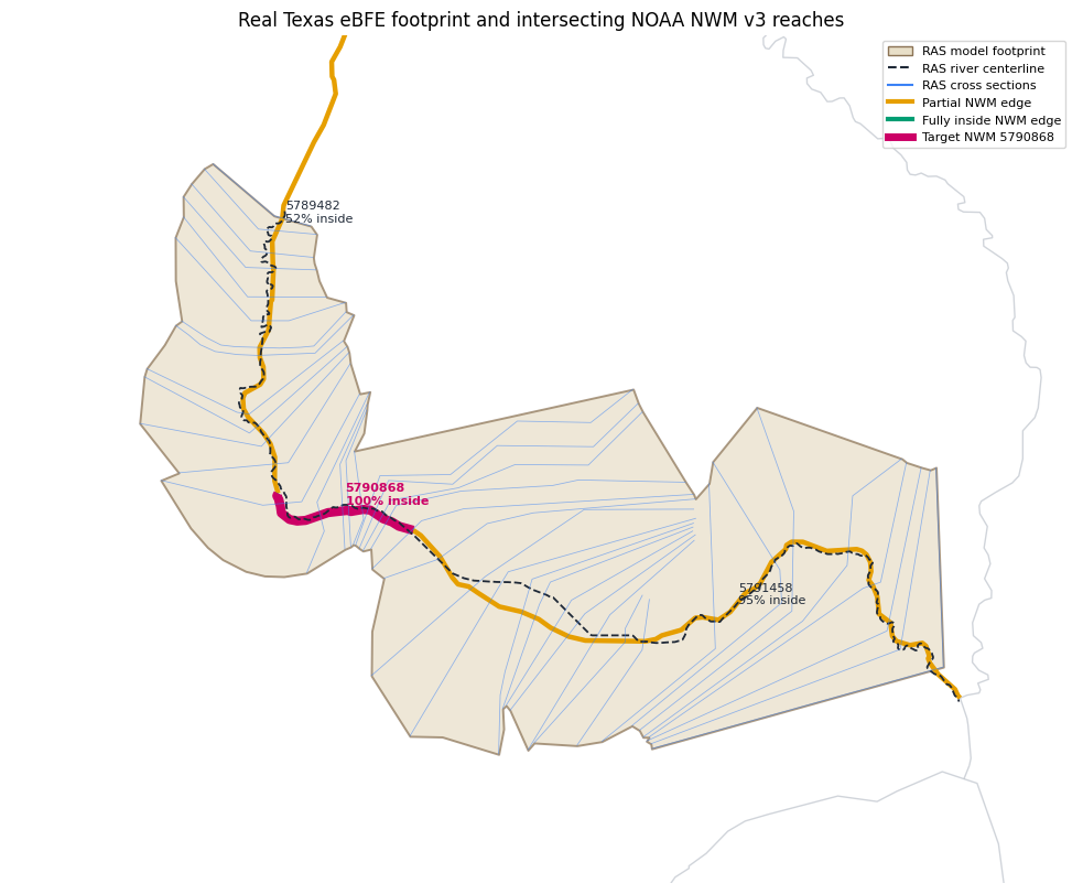
Verified execution — model extent and NWM coverage. The source model footprint contains NWM feature 5790868 completely, while the adjoining upstream and downstream flowlines are retained as partial-coverage edges. Cross sections and the HEC-RAS centerline provide the spatial check against the network.

3. Separate strict export and buffered computation domains

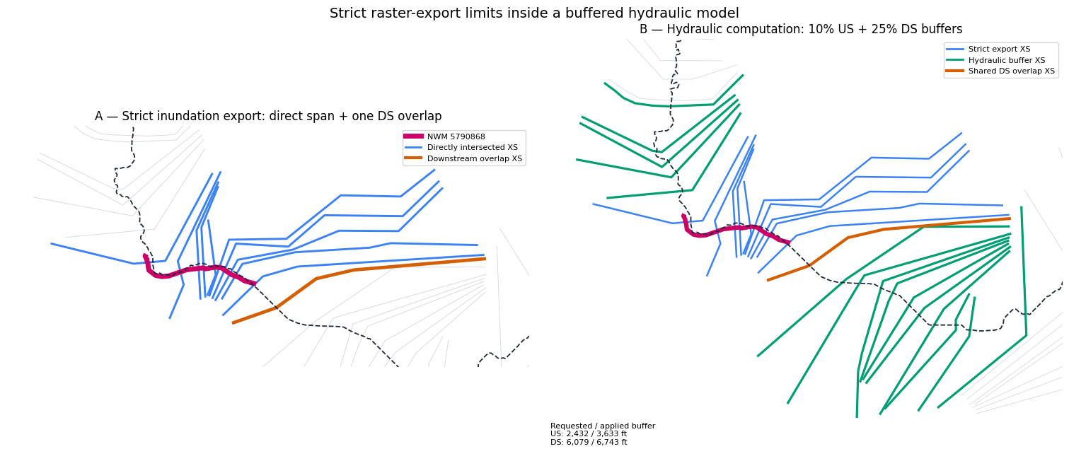
The edge intersects ten cross sections directly. Because its coverage is 100%, select_domains_by_network_edge() applies the default hydraulic buffers: 10% of the full source-reach main-channel length upstream and 25% downstream. The smaller inundation-export selection remains the direct span plus one shared downstream section, RS 14026. This keeps adjacent raster products overlapping without forcing the computation boundary against the published output limit.

Python

domains = RasBreakout1D.select_domains_by_network_edge(
    source_geometry,
    target_edge.geometry,
    river=RIVER,
    reach=REACH,
    inside_fraction=float(target_edge["inside_fraction"]),
)
direct_selection = domains.direct_selection
inundation_selection = domains.inundation_selection
selection = domains.computation_selection

direct_stations = {float(value) for value in direct_selection.stations}
inundation_stations = {float(value) for value in inundation_selection.stations}
computation_stations = {float(value) for value in selection.stations}
overlap_stations = inundation_stations - direct_stations
buffer_stations = computation_stations - inundation_stations
assert len(direct_selection.stations) == 10
assert overlap_stations == {14026.0}
assert len(inundation_selection.stations) == 11
assert len(selection.stations) == 26
assert (selection.upstream_station, selection.downstream_station) == ("21208", "8015")

source_xs["direct_intersection"] = source_xs["station_num"].isin(direct_stations)
source_xs["inundation_export"] = source_xs["station_num"].isin(inundation_stations)
source_xs["selected"] = source_xs["station_num"].isin(computation_stations)
source_xs["downstream_overlap"] = source_xs["station_num"].isin(overlap_stations)
source_xs["hydraulic_buffer"] = source_xs["station_num"].isin(buffer_stations)
direct_xs = source_xs.loc[source_xs["direct_intersection"]].copy()
overlap_xs = source_xs.loc[source_xs["downstream_overlap"]].copy()
inundation_xs = source_xs.loc[source_xs["inundation_export"]].copy()
computation_xs = source_xs.loc[source_xs["selected"]].copy()
buffer_xs = source_xs.loc[source_xs["hydraulic_buffer"]].copy()

display(pd.DataFrame({
    "nwm_edge_id": [TARGET_EDGE_ID],
    "edge_name": [target_edge["name"]],
    "main_channel_length_ft": [domains.main_channel_length],
    "directly_intersected_xs": [len(direct_selection.stations)],
    "inundation_export_xs": [len(inundation_selection.stations)],
    "overlap_xs_requested": [domains.inundation_overlap_xs],
    "overlap_xs_applied": [domains.inundation_overlap_xs_applied],
    "computation_xs": [len(selection.stations)],
    "requested_upstream_buffer_ft": [domains.upstream_buffer_distance],
    "applied_upstream_buffer_ft": [domains.upstream_buffer_applied],
    "requested_downstream_buffer_ft": [domains.downstream_buffer_distance],
    "applied_downstream_buffer_ft": [domains.downstream_buffer_applied],
    "computation_limits": [
        f"RS {selection.upstream_station} to {selection.downstream_station}"
    ],
    "inundation_limits": [
        f"RS {inundation_selection.upstream_station} to "
        f"{inundation_selection.downstream_station}"
    ],
}))

fig, axes = plt.subplots(1, 2, figsize=(15, 6.5), constrained_layout=True)

source_xs.plot(ax=axes[0], color="#D1D5DB", linewidth=0.6)
inundation_xs.plot(ax=axes[0], color=xs_color, linewidth=2.1)
overlap_xs.plot(ax=axes[0], color="#D55E00", linewidth=3.4)
gpd.GeoSeries([target_edge.geometry], crs=PROJECT_CRS).plot(
    ax=axes[0], color=target_color, linewidth=5.0
)
source_centerline.plot(ax=axes[0], color=ras_color, linewidth=1.3, linestyle="--")
strict_bounds = inundation_xs.total_bounds
strict_pad = 0.10 * max(
    strict_bounds[2] - strict_bounds[0], strict_bounds[3] - strict_bounds[1]
)
axes[0].set_xlim(strict_bounds[0] - strict_pad, strict_bounds[2] + strict_pad)
axes[0].set_ylim(strict_bounds[1] - strict_pad, strict_bounds[3] + strict_pad)
axes[0].set_title("A — Strict inundation export: direct span + one DS overlap")
axes[0].legend(
    handles=[
        Line2D([0], [0], color=target_color, linewidth=5, label=f"NWM {TARGET_EDGE_ID}"),
        Line2D([0], [0], color=xs_color, linewidth=2, label="Directly intersected XS"),
        Line2D([0], [0], color="#D55E00", linewidth=3, label="Downstream overlap XS"),
    ],
    loc="best", fontsize=8,
)

source_xs.plot(ax=axes[1], color="#D1D5DB", linewidth=0.55)
inundation_xs.plot(ax=axes[1], color=xs_color, linewidth=1.8)
buffer_xs.plot(ax=axes[1], color=inside_color, linewidth=2.3)
overlap_xs.plot(ax=axes[1], color="#D55E00", linewidth=3.0)
gpd.GeoSeries([target_edge.geometry], crs=PROJECT_CRS).plot(
    ax=axes[1], color=target_color, linewidth=4.5
)
source_centerline.plot(ax=axes[1], color=ras_color, linewidth=1.3, linestyle="--")
compute_bounds = computation_xs.total_bounds
compute_pad = 0.08 * max(
    compute_bounds[2] - compute_bounds[0], compute_bounds[3] - compute_bounds[1]
)
axes[1].set_xlim(compute_bounds[0] - compute_pad, compute_bounds[2] + compute_pad)
axes[1].set_ylim(compute_bounds[1] - compute_pad, compute_bounds[3] + compute_pad)
axes[1].set_title("B — Hydraulic computation: 10% US + 25% DS buffers")
axes[1].legend(
    handles=[
        Line2D([0], [0], color=xs_color, linewidth=2, label="Strict export XS"),
        Line2D([0], [0], color=inside_color, linewidth=2, label="Hydraulic buffer XS"),
        Line2D([0], [0], color="#D55E00", linewidth=3, label="Shared DS overlap XS"),
    ],
    loc="best", fontsize=8,
)
axes[1].text(
    0.02,
    0.02,
    f"Requested / applied buffer\n"
    f"US: {domains.upstream_buffer_distance:,.0f} / {domains.upstream_buffer_applied:,.0f} ft\n"
    f"DS: {domains.downstream_buffer_distance:,.0f} / {domains.downstream_buffer_applied:,.0f} ft",
    transform=axes[1].transAxes,
    fontsize=8,
    va="bottom",
)
for ax in axes:
    ax.set_aspect("equal")
    ax.set_axis_off()
fig.suptitle("Strict raster-export limits inside a buffered hydraulic model", fontsize=14)
plt.show()

Verified execution — nested domains. The strict export selection contains 10 directly intersected cross sections plus orange RS 14026. The buffered hydraulic model contains 26 sections from RS 21208 to RS 8015; green sections are computational overlap that will not enlarge the published raster footprint.

4. Write, validate, and run the buffered independent breakout

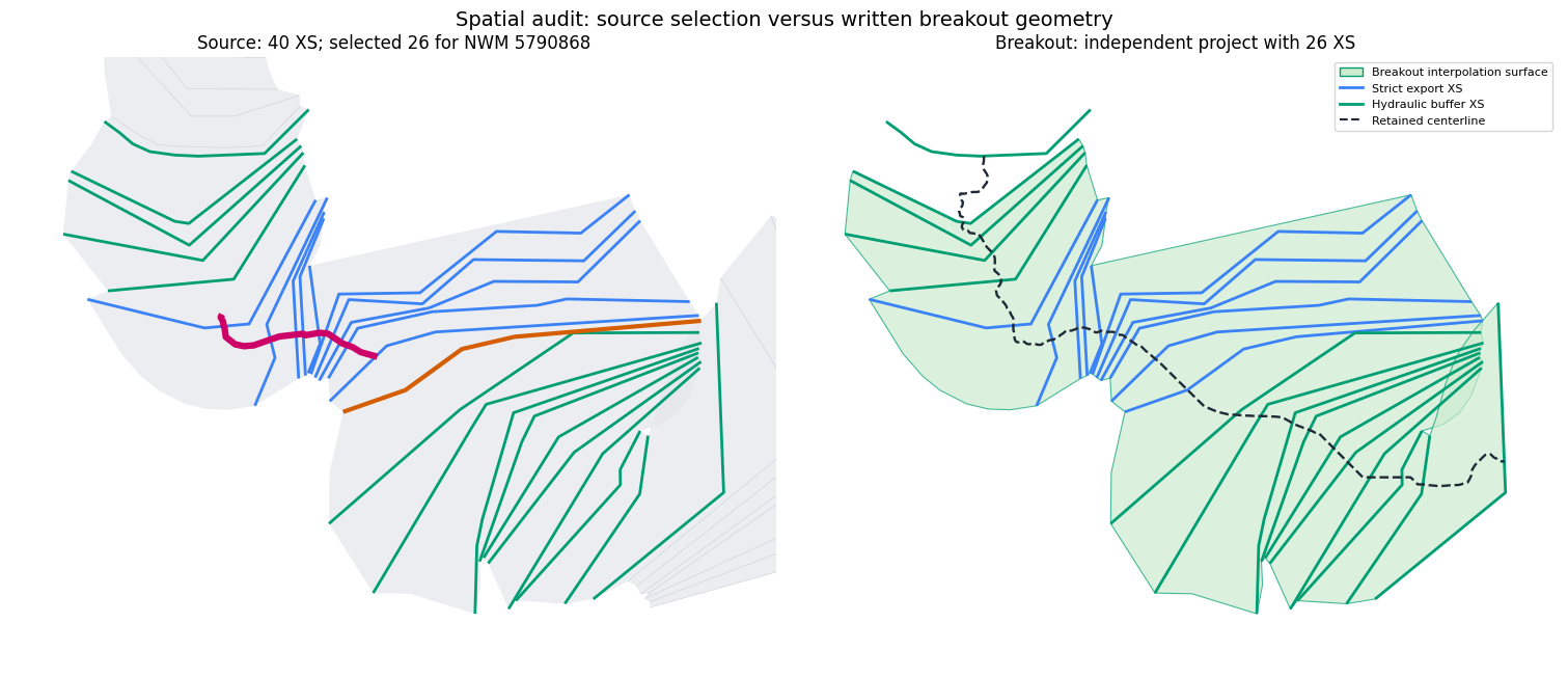
Selection and writing remain separate. The extractor copies complete retained cross-section blocks and steady-flow relationships, creates its own project, derives an internal downstream boundary from source results, and validates the destination before execution. The 26-section computation selection is written; the 11-section inundation selection remains an output-clipping contract rather than the hydraulic model boundary. HEC-RAS completes the hydraulic run and writes all expected results. Rebuilding this legacy eBFE interpolation surface also emits a nonfatal edge-line self-intersection diagnostic, which is retained in the execution audit below instead of being hidden.

Python

breakout = RasBreakout1D.extract_selection(
    source_ras,
    RUN_ROOT / f"breakout_nwm_{TARGET_EDGE_ID}",
    selection,
    plan_number=PLAN_NUMBER,
    destination_name=f"Shiloh_NWM_{TARGET_EDGE_ID}",
    source_plan_hdf=source_plan_hdf,
    boundary_mode="auto",
)

display(breakout.validation.checks_df)
assert breakout.validation.is_valid
print(f"Boundary provenance: {breakout.boundary_provenance}")
print(f"Independent project: {breakout.project_file}")

geometry_comparison = RasBreakout1D.compare_geometry(
    source_geometry,
    breakout.geometry_file,
    breakout.selection,
)
display(geometry_comparison)
assert geometry_comparison["content_equal"].all()
assert geometry_comparison.attrs["structure_blocks_equal"] is True

breakout_compute = RasBreakout1D.run(
    breakout,
    verify=False,
    force_rerun=True,
    num_cores=1,
)
assert breakout_compute, "Breakout steady plan did not complete successfully"
breakout_plan_hdf = Path(f"{breakout.plan_file}.hdf")
assert breakout_plan_hdf.is_file()
breakout_messages = HdfResultsPlan.get_compute_messages_hdf_only(
    breakout_plan_hdf
)
breakout_compute_audit = ResultsParser.parse_compute_messages(
    breakout_messages
)
assert breakout_compute_audit["completed"] is True
surface_diagnostic = breakout_compute_audit["first_error_line"] or "none"
if breakout_compute_audit["has_errors"]:
    assert "edge lines have self intersections" in surface_diagnostic.lower()
display(pd.DataFrame({
    "complete_process": [breakout_compute_audit["completed"]],
    "hydraulic_results_hdf": [breakout_plan_hdf.is_file()],
    "interpolation_surface_diagnostic": [surface_diagnostic],
}))

Python

breakout_geometry_hdf = Path(f"{breakout.geometry_file}.hdf")
breakout_xs = GeomParser.get_xs_cut_lines(breakout.geometry_file).set_crs(
    PROJECT_CRS, allow_override=True
)
breakout_centerline = GeomParser.get_river_centerlines(breakout.geometry_file).set_crs(
    PROJECT_CRS, allow_override=True
)
breakout_surface = HdfXsec.get_xs_interpolation_surface(breakout_geometry_hdf).set_crs(
    PROJECT_CRS, allow_override=True
)
selected_source_xs = source_xs.loc[source_xs["selected"]].copy()
excluded_source_xs = source_xs.loc[~source_xs["selected"]].copy()
breakout_xs["station_num"] = pd.to_numeric(
    breakout_xs["station"], errors="coerce"
)
breakout_inundation_xs = breakout_xs.loc[
    breakout_xs["station_num"].isin(inundation_stations)
].copy()
breakout_buffer_xs = breakout_xs.loc[
    ~breakout_xs["station_num"].isin(inundation_stations)
].copy()

fig, axes = plt.subplots(1, 2, figsize=(15, 6.5), constrained_layout=True)
source_surface.plot(ax=axes[0], color="#E5E7EB", edgecolor="none", alpha=0.72)
excluded_source_xs.plot(ax=axes[0], color="#9CA3AF", linewidth=0.4, alpha=0.45)
inundation_xs.plot(ax=axes[0], color=xs_color, linewidth=2.0)
buffer_xs.plot(ax=axes[0], color=inside_color, linewidth=2.0)
overlap_xs.plot(ax=axes[0], color="#D55E00", linewidth=3.0)
gpd.GeoSeries([target_edge.geometry], crs=PROJECT_CRS).plot(
    ax=axes[0], color=target_color, linewidth=4.5
)
axes[0].set_title(f"Source: 40 XS; selected {len(selected_source_xs)} for NWM {TARGET_EDGE_ID}")

breakout_surface.plot(
    ax=axes[1], color="#CDECCF", edgecolor=inside_color, linewidth=0.8, alpha=0.7
)
breakout_inundation_xs.plot(ax=axes[1], color=xs_color, linewidth=2.0)
breakout_buffer_xs.plot(ax=axes[1], color=inside_color, linewidth=2.0)
breakout_centerline.plot(ax=axes[1], color=ras_color, linewidth=1.7, linestyle="--")
axes[1].set_title(f"Breakout: independent project with {len(breakout_xs)} XS")

focus_bounds = selected_source_xs.total_bounds
focus_pad = 0.08 * max(
    focus_bounds[2] - focus_bounds[0], focus_bounds[3] - focus_bounds[1]
)
for ax in axes:
    ax.set_xlim(focus_bounds[0] - focus_pad, focus_bounds[2] + focus_pad)
    ax.set_ylim(focus_bounds[1] - focus_pad, focus_bounds[3] + focus_pad)
    ax.set_aspect("equal")
    ax.set_axis_off()
axes[1].legend(
    handles=[
        Patch(facecolor="#CDECCF", edgecolor=inside_color, label="Breakout interpolation surface"),
        Line2D([0], [0], color=xs_color, linewidth=2, label="Strict export XS"),
        Line2D([0], [0], color=inside_color, linewidth=2, label="Hydraulic buffer XS"),
        Line2D([0], [0], color=ras_color, linestyle="--", label="Retained centerline"),
    ],
    loc="best", fontsize=8,
)
fig.suptitle("Spatial audit: source selection versus written breakout geometry", fontsize=14)
plt.show()

Verified execution — written geometry. The left panel identifies the 26 retained computation sections within the 40-section source model. The right panel reads the new geometry HDF back from the standalone breakout. Blue sections support raster export; green sections are hydraulic buffer only.

5. Rasterize the computation and inundation-export domains

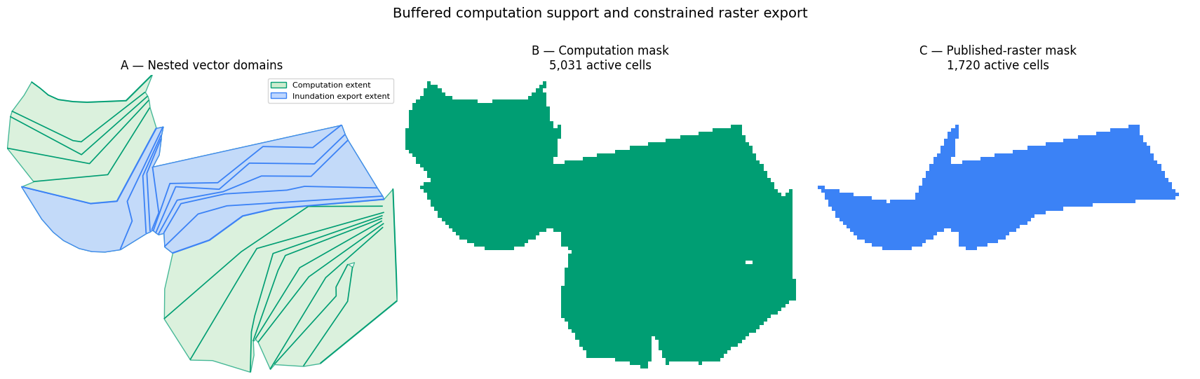
The source geometry HDF already contains interpolation-surface polygons between adjacent cross sections. Their union provides a transparent preview of the two domains without pretending that this legacy model has a registered terrain or a RAS Mapper depth grid. Both polygons are rasterized on the same 100-foot grid and written as GeoTIFF masks. A later stored-map workflow can use the smaller mask to clip depth or WSE rasters generated from the buffered model.

Python

source_hdf_xs = HdfXsec.get_cross_sections(source_geometry_hdf).reset_index(
    names="xs_id"
)
source_hdf_xs = source_hdf_xs.loc[
    (source_hdf_xs["River"] == RIVER) & (source_hdf_xs["Reach"] == REACH)
].copy()
source_hdf_xs["station_num"] = pd.to_numeric(
    source_hdf_xs["RS"], errors="coerce"
)
station_to_xs_id = source_hdf_xs.set_index("station_num")["xs_id"].to_dict()


def interpolation_extent(domain_selection):
    selected_ids = [
        int(station_to_xs_id[float(station)])
        for station in domain_selection.stations
    ]
    pairs = set(zip(selected_ids[:-1], selected_ids[1:]))
    pieces = source_surface.loc[
        source_surface.apply(
            lambda row: (int(row["us_xs_id"]), int(row["ds_xs_id"])) in pairs,
            axis=1,
        )
    ].copy()
    assert len(pieces) == len(selected_ids) - 1
    return pieces.geometry.union_all()


computation_extent = interpolation_extent(selection)
inundation_extent = interpolation_extent(inundation_selection)
outside_area = inundation_extent.difference(computation_extent).area
assert outside_area <= max(1e-6, inundation_extent.area * 1e-10)

cell_size = 100.0
xmin, ymin, xmax, ymax = computation_extent.bounds
raster_width = int(np.ceil((xmax - xmin) / cell_size))
raster_height = int(np.ceil((ymax - ymin) / cell_size))
raster_transform = from_origin(xmin, ymax, cell_size, cell_size)
raster_shape = (raster_height, raster_width)
computation_mask = rasterize(
    [(computation_extent, 1)],
    out_shape=raster_shape,
    transform=raster_transform,
    fill=0,
    dtype="uint8",
)
inundation_mask = rasterize(
    [(inundation_extent, 1)],
    out_shape=raster_shape,
    transform=raster_transform,
    fill=0,
    dtype="uint8",
)
assert 0 < inundation_mask.sum() < computation_mask.sum()

raster_profile = {
    "driver": "GTiff",
    "height": raster_height,
    "width": raster_width,
    "count": 1,
    "dtype": "uint8",
    "crs": PROJECT_CRS,
    "transform": raster_transform,
    "nodata": 0,
    "compress": "deflate",
}
computation_mask_path = RUN_ROOT / "computation_domain_mask.tif"
inundation_mask_path = RUN_ROOT / "inundation_export_domain_mask.tif"
for output_path, values in [
    (computation_mask_path, computation_mask),
    (inundation_mask_path, inundation_mask),
]:
    with rasterio.open(output_path, "w", **raster_profile) as destination:
        destination.write(values, 1)

fig, axes = plt.subplots(1, 3, figsize=(17, 6), constrained_layout=True)
gpd.GeoSeries([computation_extent], crs=PROJECT_CRS).plot(
    ax=axes[0], color="#CDECCF", edgecolor=inside_color, alpha=0.70
)
gpd.GeoSeries([inundation_extent], crs=PROJECT_CRS).plot(
    ax=axes[0], color="#BFD7FF", edgecolor=xs_color, alpha=0.85
)
buffer_xs.plot(ax=axes[0], color=inside_color, linewidth=1.2)
inundation_xs.plot(ax=axes[0], color=xs_color, linewidth=1.3)
axes[0].set_title("A — Nested vector domains")
axes[0].legend(
    handles=[
        Patch(facecolor="#CDECCF", edgecolor=inside_color, label="Computation extent"),
        Patch(facecolor="#BFD7FF", edgecolor=xs_color, label="Inundation export extent"),
    ],
    loc="best",
    fontsize=8,
)

raster_extent = [xmin, xmax, ymin, ymax]
axes[1].imshow(
    np.ma.masked_equal(computation_mask, 0),
    extent=raster_extent,
    origin="upper",
    cmap=ListedColormap([inside_color]),
    interpolation="nearest",
)
axes[1].set_title(
    f"B — Computation mask\n{int(computation_mask.sum()):,} active cells"
)
axes[2].imshow(
    np.ma.masked_equal(inundation_mask, 0),
    extent=raster_extent,
    origin="upper",
    cmap=ListedColormap([xs_color]),
    interpolation="nearest",
)
axes[2].set_title(
    f"C — Published-raster mask\n{int(inundation_mask.sum()):,} active cells"
)
for ax in axes:
    ax.set_xlim(xmin, xmax)
    ax.set_ylim(ymin, ymax)
    ax.set_aspect("equal")
    ax.set_axis_off()
fig.suptitle("Buffered computation support and constrained raster export", fontsize=14)
plt.show()

display(pd.DataFrame({
    "artifact": ["computation mask", "inundation export mask"],
    "path": [computation_mask_path, inundation_mask_path],
    "active_cells": [int(computation_mask.sum()), int(inundation_mask.sum())],
    "cell_size_ft": [cell_size, cell_size],
}))

Verified execution — rasterized output domains. Both masks share one grid. The buffered computation mask preserves transition length around NWM 5790868; the smaller published-raster mask stops at the strict 11-section selection, including its one-section downstream overlap.

6. Compare retained hydraulic results

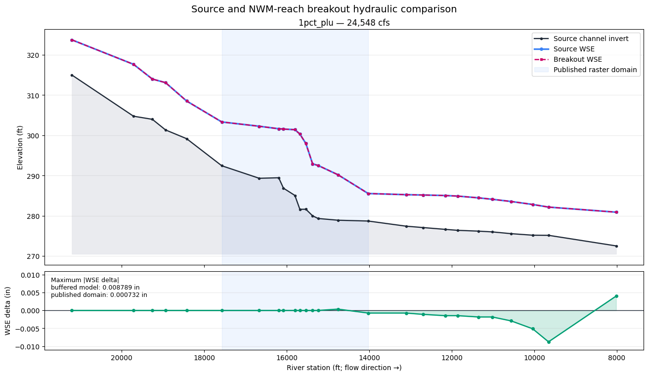
The comparison is keyed by river, reach, cross section, and profile. The figure uses the largest source flow profile and shows both the longitudinal water surface and the source-minus-breakout residual across the buffered model. The strict inundation-export range is shaded so boundary-support sections remain visually separate from the intended published result domain.

Python

results_comparison = RasBreakout1D.compare_results(
    source_plan_hdf,
    breakout_plan_hdf,
    breakout.selection,
)
assert results_comparison["_merge"].eq("both").all()
results_comparison["inundation_export"] = pd.to_numeric(
    results_comparison["node_id"], errors="coerce"
).isin(inundation_stations)
assert len(results_comparison) == 26 * 7
assert int(results_comparison["inundation_export"].sum()) == 11 * 7

delta_columns = [
    column for column in results_comparison.columns
    if column.endswith("_delta") and column != "channel_length_delta"
]
delta_summary = (
    results_comparison[delta_columns]
    .abs()
    .agg(["count", "mean", "max"])
    .T
    .sort_index()
)
display(delta_summary)

profile_flows = results_comparison.groupby("profile", observed=True)["flow_source"].max()
comparison_profile = profile_flows.idxmax()
profile_plot = results_comparison.loc[
    results_comparison["profile"] == comparison_profile
].copy()
profile_plot["station_num"] = pd.to_numeric(profile_plot["node_id"], errors="coerce")
profile_plot = profile_plot.sort_values("station_num", ascending=False)

source_profile_xs = HdfXsec.get_cross_sections(source_geometry_hdf)
source_profile_xs = source_profile_xs.loc[
    (source_profile_xs["River"] == RIVER) & (source_profile_xs["Reach"] == REACH)
].copy()
source_profile_xs["station_num"] = pd.to_numeric(source_profile_xs["RS"], errors="coerce")
source_profile_xs["channel_invert"] = source_profile_xs["station_elevation"].apply(
    lambda points: min(float(point[1]) for point in points)
)
profile_plot = profile_plot.merge(
    source_profile_xs[["station_num", "channel_invert"]],
    on="station_num",
    how="left",
)
export_upstream = float(inundation_selection.upstream_station)
export_downstream = float(inundation_selection.downstream_station)

fig, axes = plt.subplots(
    2, 1, figsize=(13, 7.5), sharex=True,
    gridspec_kw={"height_ratios": [3, 1]}, constrained_layout=True,
)
axes[0].plot(
    profile_plot["station_num"], profile_plot["channel_invert"],
    color=ras_color, linewidth=1.7, marker=".", label="Source channel invert",
)
axes[0].fill_between(
    profile_plot["station_num"], profile_plot["channel_invert"],
    profile_plot["channel_invert"].min() - 2.0,
    color="#E5E7EB", alpha=0.8,
)
axes[0].plot(
    profile_plot["station_num"], profile_plot["wsel_source"],
    color=xs_color, linewidth=2.4, marker="o", markersize=4, label="Source WSE",
)
axes[0].plot(
    profile_plot["station_num"], profile_plot["wsel_destination"],
    color=target_color, linewidth=1.8, linestyle="--", marker="s", markersize=3.5,
    label="Breakout WSE",
)
axes[0].axvspan(
    export_downstream,
    export_upstream,
    color=xs_color,
    alpha=0.08,
    label="Published raster domain",
)
axes[0].set_ylabel("Elevation (ft)")
axes[0].set_title(
    f"{comparison_profile} — {profile_flows.loc[comparison_profile]:,.0f} cfs"
)
axes[0].ticklabel_format(style="plain", axis="y", useOffset=False)
axes[0].grid(axis="y", alpha=0.25)
axes[0].legend(loc="best")

wse_delta_inches = profile_plot["wsel_delta"] * 12.0
axes[1].axhline(0.0, color=ras_color, linewidth=1.0)
axes[1].plot(
    profile_plot["station_num"], wse_delta_inches,
    color=inside_color, linewidth=1.8, marker="o", markersize=4,
)
axes[1].fill_between(
    profile_plot["station_num"], 0.0, wse_delta_inches,
    color=inside_color, alpha=0.18,
)
axes[1].axvspan(
    export_downstream,
    export_upstream,
    color=xs_color,
    alpha=0.08,
)
axes[1].set_ylabel("WSE delta (in)")
axes[1].set_xlabel("River station (ft; flow direction →)")
axes[1].grid(axis="y", alpha=0.25)
axes[1].invert_xaxis()
max_delta_inches = float(wse_delta_inches.abs().max())
export_delta_inches = float(
    wse_delta_inches.loc[profile_plot["station_num"].isin(inundation_stations)]
    .abs()
    .max()
)
delta_limit = max(max_delta_inches * 1.25, 0.001)
axes[1].set_ylim(-delta_limit, delta_limit)
axes[1].text(
    0.01,
    0.93,
    f"Maximum |WSE delta|\n"
    f"buffered model: {max_delta_inches:.6f} in\n"
    f"published domain: {export_delta_inches:.6f} in",
    transform=axes[1].transAxes, va="top", fontsize=9,
)
fig.suptitle("Source and NWM-reach breakout hydraulic comparison", fontsize=14)
plt.show()

display(results_comparison[[
    "river", "reach", "node_id", "profile",
    "flow_source", "flow_destination", "flow_delta",
    "wsel_source", "wsel_destination", "wsel_delta",
    "inundation_export", "_merge",
]].head(18))

Verified execution — hydraulic agreement. The source and breakout water surfaces overlay for the highest-flow profile. The lower panel exposes the source-minus-breakout residual in inches rather than hiding it beneath the WSE lines. All 182 buffered-model records were present in both runs; the blue band identifies the 77 records within the constrained inundation-export domain.

Result

The destination is a standalone 1D steady HEC-RAS project for NWM feature 5790868. Its hydraulic model retains 26 sections: the ten directly intersected sections, one shared downstream export-overlap section, and 15 additional boundary-support sections. The published raster domain remains constrained to the 11-section strict selection. Both selections, their vector extents, and their aligned GeoTIFF masks are explicit and auditable.

This is the intended relationship between conflation and trimming: model extent finds the in-domain edge; the buffered selection defines the hydraulic computation; the strict overlapping selection defines the raster export footprint.