2D Spatial Result Queries with HdfResultsQuery
Query water surface elevation, depth, and velocity at arbitrary (x,y) coordinates, extract profiles along transects, compute flood extent with engineering filters, and generate domain-wide statistics -- all using scipy KDTree spatial indexing.
from ras_commander import *
from ras_commander.hdf import HdfResultsQuery
from pathlib import Path

import numpy as np
import pandas as pd
import matplotlib.pyplot as plt

plt.style.use("seaborn-v0_8-whitegrid")
pd.set_option("display.max_columns", 20)
pd.set_option("display.width", 120)
Setup and Project Extraction
Use the reproducible BaldEagleCrkMulti2D example project, initialize it with ras-commander,
and compute plan 06 before issuing any spatial queries. The notebook uses plan numbers
directly so the decorators resolve the plan HDF and companion geometry HDF for us.
PROJECT_NAME = "BaldEagleCrkMulti2D"
PLAN_NUMBER = "06"
PROJECT_SUFFIX = "415"
RAS_VERSION_OR_PATH = "7.0"  # Replace with a full Ras.exe path if needed.

try:
    from _notebook_prereqs import ensure_plan_result_hdf, get_or_extract_example_project
except ModuleNotFoundError:
    import sys

    examples_dir = Path.cwd() if Path.cwd().name == "examples" else Path.cwd() / "examples"
    if examples_dir.exists() and str(examples_dir) not in sys.path:
        sys.path.insert(0, str(examples_dir))
    from _notebook_prereqs import ensure_plan_result_hdf, get_or_extract_example_project

project_path = get_or_extract_example_project(PROJECT_NAME, suffix=PROJECT_SUFFIX)
init_ras_project(project_path, RAS_VERSION_OR_PATH)

# Ensure the required results HDF is present before analysis cells run.
_plan_hdf_check = ensure_plan_result_hdf(
    PLAN_NUMBER,
    ras_object=ras,
    num_cores=2,
    clear_geompre=False,
)

plan_columns = [
    col for col in ["plan_number", "plan_title", "Geom File", "HDF_Results_Path"]
    if col in ras.plan_df.columns
]
plan_overview = ras.plan_df.loc[:, plan_columns].copy()
plan_overview["plan_number"] = plan_overview["plan_number"].astype(str).str.zfill(2)

plan_hdf = Path(_plan_hdf_check)

print(f"Project folder: {project_path}")
print(f"Plan HDF: {plan_hdf.name}")
plan_overview.head()
2026-06-11 16:52:28 - ras_commander.RasExamples - INFO - Successfully extracted project 'BaldEagleCrkMulti2D' to <workspace>\examples\example_projects\BaldEagleCrkMulti2D_415


2026-06-11 16:52:28 - ras_commander.RasUtils - INFO - Discovered HEC-RAS 7.0 at <hec_ras_install>\7.0\Ras.exe via filesystem (x86)


2026-06-11 16:52:28 - ras_commander.RasUtils - INFO - Discovered HEC-RAS 6.7 Beta 5 at <hec_ras_install>\6.7 Beta 5\Ras.exe via filesystem (x86)


2026-06-11 16:52:28 - ras_commander.RasUtils - INFO - Discovered HEC-RAS 6.6 at <hec_ras_install>\6.6\Ras.exe via filesystem (x86)


2026-06-11 16:52:28 - ras_commander.RasUtils - INFO - Discovered HEC-RAS 6.5 at <hec_ras_install>\6.5\Ras.exe via filesystem (x86)


2026-06-11 16:52:28 - ras_commander.RasUtils - INFO - Discovered HEC-RAS 6.4.1 at <hec_ras_install>\6.4.1\Ras.exe via filesystem (x86)


2026-06-11 16:52:28 - ras_commander.RasUtils - INFO - Discovered HEC-RAS 6.3.1 at <hec_ras_install>\6.3.1\Ras.exe via filesystem (x86)


2026-06-11 16:52:28 - ras_commander.RasUtils - INFO - Discovered HEC-RAS 6.3 at <hec_ras_install>\6.3\Ras.exe via filesystem (x86)


2026-06-11 16:52:28 - ras_commander.RasUtils - INFO - Discovered HEC-RAS 6.2 at <hec_ras_install>\6.2\Ras.exe via filesystem (x86)


2026-06-11 16:52:28 - ras_commander.RasUtils - INFO - Discovered HEC-RAS 6.1 at <hec_ras_install>\6.1\Ras.exe via filesystem (x86)


2026-06-11 16:52:28 - ras_commander.RasUtils - INFO - Discovered HEC-RAS 6.0 at <hec_ras_install>\6.0\Ras.exe via filesystem (x86)


2026-06-11 16:52:28 - ras_commander.RasUtils - INFO - Discovered HEC-RAS 5.0.7 at <hec_ras_install>\5.0.7\Ras.exe via filesystem (x86)


2026-06-11 16:52:28 - ras_commander.RasUtils - INFO - Discovered HEC-RAS 5.0.6 at <hec_ras_install>\5.0.6\Ras.exe via filesystem (x86)


2026-06-11 16:52:28 - ras_commander.RasUtils - INFO - Discovered HEC-RAS 5.0.3 at <hec_ras_install>\5.0.3\Ras.exe via filesystem (x86)


2026-06-11 16:52:28 - ras_commander.RasUtils - INFO - Discovered HEC-RAS 4.1.0 at <hec_ras_install>\4.1.0\Ras.exe via filesystem (x86)


2026-06-11 16:52:28 - ras_commander.RasUtils - INFO - Discovered HEC-RAS 4.0 at <hec_ras_install>\4.0\Ras.exe via filesystem (x86)


2026-06-11 16:52:28 - ras_commander.RasUtils - INFO - Discovered HEC-RAS 6.7 Beta 4a at <hec_ras_install>\6.7 Beta 4a\Ras.exe via filesystem (x86)


2026-06-11 16:52:28 - ras_commander.RasUtils - INFO - Discovered 16 installed HEC-RAS version(s)


2026-06-11 16:52:28 - ras_commander.RasPrj - INFO - HEC-RAS 7.0 found via version discovery: <hec_ras_install>\7.0\Ras.exe


2026-06-11 16:52:28 - ras_commander.RasMap - INFO - Successfully parsed RASMapper file: <workspace>\examples\example_projects\BaldEagleCrkMulti2D_415\BaldEagleDamBrk.rasmap


2026-06-11 16:52:28 - ras_commander.RasPrj - INFO - ras-commander v0.98.0 | An open-source project of CLB Engineering Corporation (https://clbengineering.com/) | Docs: https://rascommander.info | GitHub: https://github.com/gpt-cmdr/ras-commander


2026-06-11 16:52:28 - ras_commander.RasPrj - INFO - Project initialized: BaldEagleDamBrk | Folder: <workspace>\examples\example_projects\BaldEagleCrkMulti2D_415


2026-06-11 16:52:28 - ras_commander.RasPrj - INFO - Using HEC-RAS executable: <hec_ras_install>\7.0\Ras.exe


2026-06-11 16:52:28 - ras_commander.RasPrj - INFO -
═══════════════════════════════════════════════════════════════════════
ras-commander | HEC-RAS Automation Library
Docs: https://rascommander.info/
Repo: https://github.com/gpt-cmdr/ras-commander
═══════════════════════════════════════════════════════════════════════

PROJECT DATAFRAMES (single source of truth — use these, not file globbing):
  ras.plan_df        Plans, HDF paths, geometry/flow associations
  ras.geom_df        Geometry files and HDF preprocessor paths
  ras.flow_df        Steady flow files
  ras.unsteady_df    Unsteady flow files and configurations
  ras.boundaries_df  Boundary conditions (type, name, location)
  ras.results_df     Lightweight HDF results summaries
  ras.rasmap_df      RASMapper layers, terrain, land cover paths

KEY APIS (static classes — call directly, never instantiate):
  Execution:    RasCmdr.compute_plan() / compute_parallel() / compute_test_mode()
  Plan Files:   RasPlan.clone_plan() / clone_geom() / set_geom()
  Unsteady:     RasUnsteady — IC/BC management, gate openings, precipitation
  Geometry:     GeomCrossSection, GeomBridge, GeomStorage, GeomLateral, GeomMesh
  HDF Results:  HdfResultsPlan.get_wse() / get_compute_messages()
                HdfResultsMesh.get_mesh_max_ws() / get_mesh_cells_timeseries()
                HdfMesh.get_mesh_cell_points()
  QA/QC:        RasCheck.run_check() / RasFixit (geometry repair)
  DSS:          RasDss.get_timeseries() / check_pathname()
  USGS:         UsgsGaugeSpatial, GaugeMatcher, RasUsgsBoundaryGeneration
  Precipitation: StormGenerator, Atlas14Storm, PrecipAorc, Atlas14Variance
  Terrain:      RasTerrain.create_terrain_hdf() / RasTerrainMod

MULTI-PROJECT: Pass ras_object= to all API calls when using local RasPrj instances.

EXAMPLES: 100+ notebooks in examples/ (100s=execution, 200s=geometry, 300s=unsteady,
  400s=HDF results, 500s=remote, 800s=QA/QC, 900s=data integration).
  Review relevant notebooks before assembling new workflows.

PLATFORM: Most HEC-RAS operations require Windows. Linux/Wine support for
  headless execution, data access, geometry modification, and preprocessing
  is available via RasProcess (HEC-RAS 6.6+). See ras_commander/RasProcess.py.
  Remote distributed execution: ras_commander/remote/ (PsExec, Docker, SSH, cloud).
═══════════════════════════════════════════════════════════════════════


2026-06-11 16:52:28 - ras_commander.RasCmdr - INFO - Using ras_object with project folder: <workspace>\examples\example_projects\BaldEagleCrkMulti2D_415


2026-06-11 16:52:28 - ras_commander.RasUtils - INFO - Successfully updated file: <workspace>\examples\example_projects\BaldEagleCrkMulti2D_415\BaldEagleDamBrk.p06


Plan 06 HDF is missing; computing prerequisite: <workspace>\examples\example_projects\BaldEagleCrkMulti2D_415\BaldEagleDamBrk.p06.hdf


2026-06-11 16:52:28 - ras_commander.RasCmdr - INFO - Set number of cores to 2 for plan: 06


2026-06-11 16:52:28 - ras_commander.RasCmdr - INFO - Running HEC-RAS from the Command Line:


2026-06-11 16:52:28 - ras_commander.RasCmdr - INFO - Running command: "<hec_ras_install>\7.0\Ras.exe" -c "<workspace>\examples\example_projects\BaldEagleCrkMulti2D_415\BaldEagleDamBrk.prj" "<workspace>\examples\example_projects\BaldEagleCrkMulti2D_415\BaldEagleDamBrk.p06"


2026-06-11 16:52:28 - ras_commander.RasDialogWatchdog - INFO - DialogWatchdog started — polling every 1.5s for RAS dialog windows


2026-06-11 16:57:52 - ras_commander.RasCmdr - INFO - HEC-RAS execution completed for plan: 06


2026-06-11 16:57:52 - ras_commander.RasCmdr - INFO - Total run time for plan 06: 323.20 seconds


2026-06-11 16:57:52 - ras_commander.RasDialogWatchdog - INFO - DialogWatchdog stopped — no dialogs encountered


Project folder: <workspace>\examples\example_projects\BaldEagleCrkMulti2D_415
Plan HDF: BaldEagleDamBrk.p06.hdf
| plan_number | Geom File | HDF_Results_Path | |
|---|---|---|---|
| 0 | 13 | 06 | NaN |
| 1 | 15 | 08 | NaN |
| 2 | 17 | 10 | NaN |
| 3 | 18 | 11 | NaN |
| 4 | 19 | 12 | NaN |
Build Reproducible Query Locations
Rather than hard-coding coordinates, pull maximum-depth and maximum-WSE envelopes, keep wet cells, and reuse those cell-center coordinates for point, batch, and profile queries. This keeps the notebook reproducible even if the extracted project folder changes.
# get_mesh_max_ws returns cell-center GeoDataFrame with max WSE values
max_wse_gdf = HdfResultsMesh.get_mesh_max_ws(PLAN_NUMBER)

# Compute max depth from WSE and cell minimum elevation (from geometry HDF)
import h5py

geom_number = ras.plan_df.loc[
    ras.plan_df["plan_number"].astype(str).str.zfill(2) == PLAN_NUMBER,
    "Geom File",
].iloc[0]
geom_hdf_path = ras.project_folder / f"{ras.project_name}.g{str(geom_number).zfill(2)}.hdf"

cell_min_elev = {}
with h5py.File(geom_hdf_path, "r") as gf:
    base = "Geometry/2D Flow Areas"
    for mesh_name in gf[base]:
        elev_path = f"{base}/{mesh_name}/Cells Minimum Elevation"
        if elev_path in gf:
            cell_min_elev[mesh_name] = gf[elev_path][()]

# Add minimum elevation to GeoDataFrame and compute depth
elev_series = []
for _, row in max_wse_gdf.iterrows():
    mesh = row["mesh_name"]
    cid = int(row["cell_id"])
    if mesh in cell_min_elev and cid < len(cell_min_elev[mesh]):
        elev_series.append(float(cell_min_elev[mesh][cid]))
    else:
        elev_series.append(float("nan"))

max_wse_gdf["cell_min_elevation"] = elev_series
max_wse_gdf["maximum_depth"] = (
    max_wse_gdf["maximum_water_surface"] - max_wse_gdf["cell_min_elevation"]
).clip(lower=0)

analysis_cells = max_wse_gdf.assign(
    x=lambda df: df.geometry.x,
    y=lambda df: df.geometry.y,
)

wet_cells = analysis_cells.loc[analysis_cells["maximum_depth"] > 0.5].copy()
if wet_cells.empty:
    wet_cells = analysis_cells.nlargest(12, "maximum_depth").copy()

wet_cells = wet_cells.sort_values(["mesh_name", "x"]).reset_index(drop=True)
sample_count = min(6, len(wet_cells))
sample_index = np.linspace(0, len(wet_cells) - 1, sample_count, dtype=int)
sample_points = wet_cells.iloc[np.unique(sample_index)].copy().reset_index(drop=True)
sample_points["point_id"] = [f"P{i+1}" for i in range(len(sample_points))]

mesh_for_profile = sample_points["mesh_name"].mode().iloc[0]
profile_pool = wet_cells.loc[wet_cells["mesh_name"] == mesh_for_profile].reset_index(drop=True)
if len(profile_pool) < 2:
    profile_pool = analysis_cells.reset_index(drop=True)
if len(profile_pool) < 2:
    raise ValueError("Need at least two cell centers to build a profile transect")

# Use a local transect between neighboring wet cell centers to avoid sampling outside the mesh.
anchor_idx = len(profile_pool) // 2
anchor = profile_pool.iloc[anchor_idx]
neighbor_distances = (profile_pool["x"] - anchor["x"]) ** 2 + (profile_pool["y"] - anchor["y"]) ** 2
neighbor_distances.iloc[anchor_idx] = np.inf
neighbor_idx = int(neighbor_distances.idxmin())
profile_start = anchor
profile_end = profile_pool.loc[neighbor_idx]

sample_points[
    ["point_id", "mesh_name", "cell_id", "x", "y", "maximum_depth", "maximum_water_surface"]
].head()
2026-06-11 16:57:52 - ras_commander.hdf.HdfResultsMesh - INFO - Processed 19597 rows of summary output data
| point_id | mesh_name | cell_id | x | y | maximum_depth | maximum_water_surface | |
|---|---|---|---|---|---|---|---|
| 0 | P1 | BaldEagleCr | 17613 | 1966250.0 | 292000.0 | 4.550476 | 768.610779 |
| 1 | P2 | BaldEagleCr | 14946 | 1998500.0 | 312500.0 | 58.539307 | 659.783203 |
| 2 | P3 | BaldEagleCr | 11378 | 2017750.0 | 330750.0 | 3.652222 | 598.704529 |
| 3 | P4 | BaldEagleCr | 8010 | 2039750.0 | 342250.0 | 1.056152 | 579.192444 |
| 4 | P5 | BaldEagleCr | 4326 | 2056750.0 | 354500.0 | 4.304932 | 540.370605 |
Point Query
query_point() snaps an arbitrary coordinate to the nearest 2D cell center and returns a compact
dictionary with the value, mesh name, cell id, and snap distance. Using time_index="max" makes
the first example land on the peak envelope instead of the final saved timestep.
representative_point = sample_points.iloc[len(sample_points) // 2]
print(
    f"Using {representative_point['point_id']} on {representative_point['mesh_name']} "
    f"at ({representative_point['x']:.2f}, {representative_point['y']:.2f})"
)

point_result = HdfResultsQuery.query_point(
    PLAN_NUMBER,
    x=float(representative_point["x"]),
    y=float(representative_point["y"]),
    variable="wse",
    time_index="max",
)

point_result
Using P4 on BaldEagleCr at (2039750.00, 342250.00)


2026-06-11 16:57:53 - ras_commander.hdf.HdfResultsMesh - INFO - Processed 19597 rows of summary output data


{'value': 579.1924438476562,
 'cell_id': 8010,
 'mesh_name': 'BaldEagleCr',
 'distance': 0.0,
 'x': 2039750.0,
 'y': 342250.0}
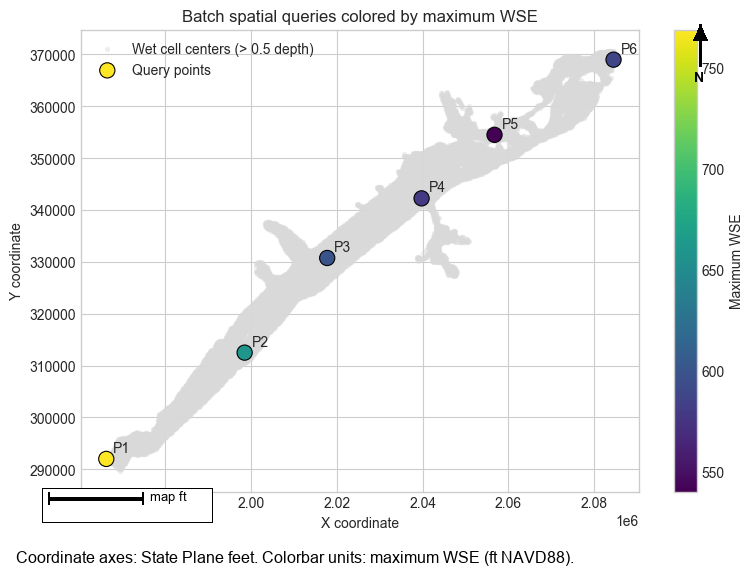
Batch Point Query
query_points() handles many coordinates in one call and returns a tidy DataFrame. Here we query
several wet-cell centers and use the maximum water-surface envelope so every sample is on the same
peak-result basis.
batch_results = (
    HdfResultsQuery.query_points(
        PLAN_NUMBER,
        sample_points[["x", "y"]].to_numpy(),
        variable="wse",
        time_index="max",
    )
    .rename(columns={"value": "wse_max"})
    .assign(point_id=sample_points["point_id"].values)
)

batch_results = batch_results[
    ["point_id", "x", "y", "mesh_name", "cell_id", "distance", "wse_max"]
]
batch_results.head()
2026-06-11 16:57:53 - ras_commander.hdf.HdfResultsMesh - INFO - Processed 19597 rows of summary output data
| point_id | x | y | mesh_name | cell_id | distance | wse_max | |
|---|---|---|---|---|---|---|---|
| 0 | P1 | 1966250.0 | 292000.0 | BaldEagleCr | 17613 | 0.0 | 768.610779 |
| 1 | P2 | 1998500.0 | 312500.0 | BaldEagleCr | 14946 | 0.0 | 659.783203 |
| 2 | P3 | 2017750.0 | 330750.0 | BaldEagleCr | 11378 | 0.0 | 598.704529 |
| 3 | P4 | 2039750.0 | 342250.0 | BaldEagleCr | 8010 | 0.0 | 579.192444 |
| 4 | P5 | 2056750.0 | 354500.0 | BaldEagleCr | 4326 | 0.0 | 540.370605 |
fig, ax = plt.subplots(figsize=(9, 6))
ax.scatter(
    wet_cells["x"],
    wet_cells["y"],
    s=8,
    color="#d9d9d9",
    alpha=0.35,
    label="Wet cell centers (> 0.5 depth)",
)
scatter = ax.scatter(
    batch_results["x"],
    batch_results["y"],
    c=batch_results["wse_max"],
    s=120,
    cmap="viridis",
    edgecolor="black",
    linewidth=0.8,
    label="Query points",
)

for row in batch_results.itertuples():
    ax.annotate(row.point_id, (row.x, row.y), xytext=(5, 5), textcoords="offset points")

ax.set_title("Batch spatial queries colored by maximum WSE")
ax.set_xlabel("X coordinate")
ax.set_ylabel("Y coordinate")
ax.legend(loc="best")
fig.colorbar(scatter, ax=ax, label="Maximum WSE")
plt.show()
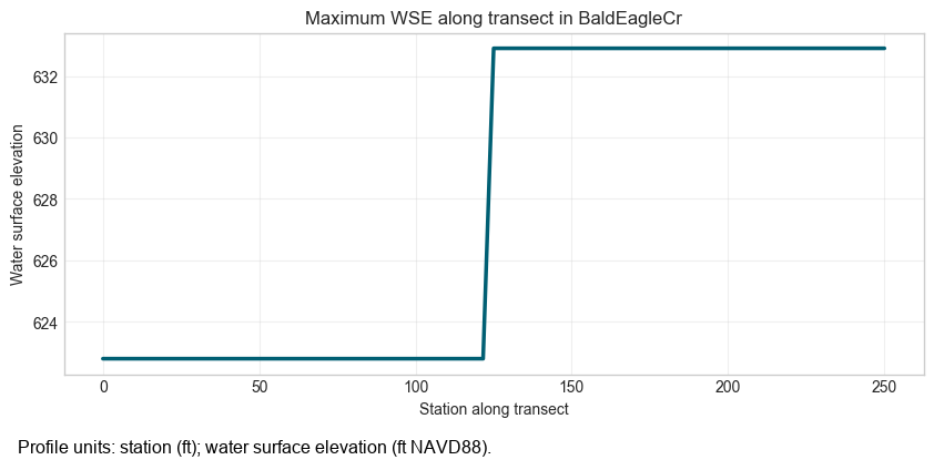
Profile Extraction
query_profile() samples evenly spaced points along a transect. The start and end points below are
taken from wet cells in the dominant mesh so the section crosses the active flow area without
hard-coded coordinates.
profile_df = HdfResultsQuery.query_profile(
    PLAN_NUMBER,
    x1=float(profile_start["x"]),
    y1=float(profile_start["y"]),
    x2=float(profile_end["x"]),
    y2=float(profile_end["y"]),
    variable="wse",
    n_points=75,
    time_index="max",
)

display(profile_df.head())

fig, ax = plt.subplots(figsize=(10, 4))
ax.plot(profile_df["station"], profile_df["value"], color="#005f73", linewidth=2.5)
ax.set_title(f"Maximum WSE along transect in {mesh_for_profile}")
ax.set_xlabel("Station along transect")
ax.set_ylabel("Water surface elevation")
ax.grid(True, alpha=0.3)
plt.show()
2026-06-11 16:57:54 - ras_commander.hdf.HdfResultsMesh - INFO - Processed 19597 rows of summary output data
| station | x | y | value | cell_id | mesh_name | distance | |
|---|---|---|---|---|---|---|---|
| 0 | 0.000000 | 2.029750e+06 | 341750.0 | 622.795959 | 8088 | BaldEagleCr | 0.000000 |
| 1 | 3.378378 | 2.029747e+06 | 341750.0 | 622.795959 | 8088 | BaldEagleCr | 3.378378 |
| 2 | 6.756757 | 2.029743e+06 | 341750.0 | 622.795959 | 8088 | BaldEagleCr | 6.756757 |
| 3 | 10.135135 | 2.029740e+06 | 341750.0 | 622.795959 | 8088 | BaldEagleCr | 10.135135 |
| 4 | 13.513514 | 2.029736e+06 | 341750.0 | 622.795959 | 8088 | BaldEagleCr | 13.513514 |
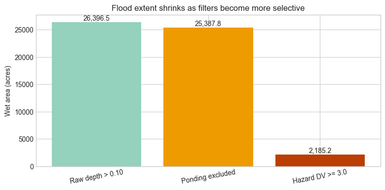
Flood Extent Analysis
flood_extent() can do more than a simple depth screen. The three cases below show raw depth,
a shallow ponding exclusion intended for rain-on-grid screening, and a hazard-oriented filter using
depth x velocity >= 3.0. For this example project the ponding filter is illustrative rather than
a calibrated rainfall-depth threshold.
raw_extent = HdfResultsQuery.flood_extent(
    PLAN_NUMBER,
    depth_threshold=0.10,
    time_index="max",
)

filtered_extent = HdfResultsQuery.flood_extent(
    PLAN_NUMBER,
    depth_threshold=0.10,
    precip_depth_threshold=0.25,
    ponding_velocity_max=0.10,
    time_index="max",
)

hazard_extent = HdfResultsQuery.flood_extent(
    PLAN_NUMBER,
    depth_threshold=0.50,
    dv_threshold=3.0,
    precip_depth_threshold=0.25,
    ponding_velocity_max=0.10,
    time_index="max",
)

extent_comparison = pd.DataFrame(
    [
        {"scenario": "Raw depth > 0.10", **raw_extent},
        {"scenario": "Ponding excluded", **filtered_extent},
        {"scenario": "Hazard DV >= 3.0", **hazard_extent},
    ]
)

# Display only columns that exist (some filters add extra keys)
display_cols = ["scenario", "wet_cells", "wet_fraction", "wet_area_acres",
                "max_depth", "mean_wet_depth"]
for optional_col in ["ponding_excluded_cells", "max_dv", "filters_applied"]:
    if optional_col in extent_comparison.columns:
        display_cols.append(optional_col)

display(extent_comparison[display_cols])

fig, ax = plt.subplots(figsize=(9, 4))
bars = ax.bar(
    extent_comparison["scenario"],
    extent_comparison["wet_area_acres"],
    color=["#94d2bd", "#ee9b00", "#bb3e03"],
)
ax.set_title("Flood extent shrinks as filters become more selective")
ax.set_ylabel("Wet area (acres)")
for bar in bars:
    height = bar.get_height()
    ax.text(
        bar.get_x() + bar.get_width() / 2,
        height,
        f"{height:,.1f}",
        ha="center",
        va="bottom",
    )
plt.xticks(rotation=10)
plt.show()
2026-06-11 16:57:54 - ras_commander.hdf.HdfResultsMesh - INFO - Processed 19597 rows of summary output data


2026-06-11 16:57:54 - ras_commander.hdf.HdfResultsMesh - INFO - Processed 19597 rows of summary output data


2026-06-11 16:57:55 - ras_commander.hdf.HdfResultsMesh - INFO - Processed 37594 rows of summary output data


2026-06-11 16:57:55 - ras_commander.hdf.HdfResultsMesh - INFO - Processed 19597 rows of summary output data


2026-06-11 16:57:56 - ras_commander.hdf.HdfResultsMesh - INFO - Processed 37594 rows of summary output data
| scenario | wet_cells | wet_fraction | wet_area_acres | max_depth | mean_wet_depth | ponding_excluded_cells | max_dv | filters_applied | |
|---|---|---|---|---|---|---|---|---|---|
| 0 | Raw depth > 0.10 | 18063 | 0.921723 | 26396.497386 | 75.082458 | 7.437328 | NaN | NaN | [depth_threshold] |
| 1 | Ponding excluded | 17360 | 0.885850 | 25387.750422 | 75.082458 | 7.731733 | 706.0 | NaN | [depth_threshold, precip_depth_threshold] |
| 2 | Hazard DV >= 3.0 | 1525 | 0.077818 | 2185.227228 | 75.082458 | 22.978986 | 706.0 | 225.207385 | [depth_threshold, dv_threshold, precip_depth_t... |
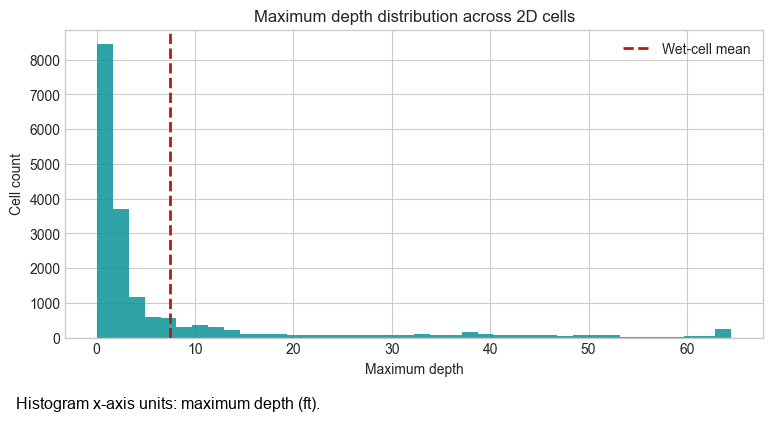
Domain Statistics
result_statistics() collapses an entire field into a compact summary. Comparing wet_only=True
and wet_only=False makes it obvious how dry cells pull the distribution toward zero.
stats_all = HdfResultsQuery.result_statistics(
    PLAN_NUMBER,
    variable="depth",
    time_index="max",
    wet_only=False,
)

stats_wet = HdfResultsQuery.result_statistics(
    PLAN_NUMBER,
    variable="depth",
    time_index="max",
    wet_only=True,
    depth_threshold=0.10,
)

stats_df = pd.DataFrame(
    [stats_all, stats_wet],
    index=["All cells", "Wet cells only"],
).T
display(stats_df.loc[["count", "min", "p10", "p25", "mean", "median", "p75", "p90", "p99", "max", "std"]])

# Clip the extreme tail so the histogram stays readable.
plot_depths = analysis_cells["maximum_depth"].clip(
    upper=analysis_cells["maximum_depth"].quantile(0.99)
)

fig, ax = plt.subplots(figsize=(9, 4))
ax.hist(plot_depths, bins=40, color="#0a9396", alpha=0.85)
ax.axvline(stats_wet["mean"], color="#ae2012", linestyle="--", linewidth=2, label="Wet-cell mean")
ax.set_title("Maximum depth distribution across 2D cells")
ax.set_xlabel("Maximum depth")
ax.set_ylabel("Cell count")
ax.legend()
plt.show()
2026-06-11 16:57:56 - ras_commander.hdf.HdfResultsMesh - INFO - Processed 19597 rows of summary output data


2026-06-11 16:57:56 - ras_commander.hdf.HdfResultsMesh - INFO - Processed 19597 rows of summary output data
| All cells | Wet cells only | |
|---|---|---|
| count | 18066.000000 | 18063.000000 |
| min | 0.053284 | 0.100098 |
| p10 | 0.478973 | 0.479333 |
| p25 | 0.892593 | 0.892761 |
| mean | 7.436105 | 7.437328 |
| median | 1.815491 | 1.816162 |
| p75 | 5.520294 | 5.523071 |
| p90 | 25.974152 | 25.975378 |
| p99 | 64.502979 | 64.503945 |
| max | 75.082458 | 75.082458 |
| std | 13.736565 | 13.737378 |
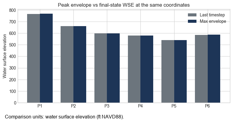
Max Envelope vs Time Step
The same coordinate can answer two different questions. time_index=-1 asks for the model state at
the final saved timestep, while time_index="max" asks for the peak envelope at that location over
the full run. Comparing both at the same sample points highlights recession between the peak and the
last output.
last_step_results = HdfResultsQuery.query_points(
    PLAN_NUMBER,
    sample_points[["x", "y"]].to_numpy(),
    variable="wse",
    time_index=-1,
).rename(columns={"value": "wse_last"})

max_envelope_results = HdfResultsQuery.query_points(
    PLAN_NUMBER,
    sample_points[["x", "y"]].to_numpy(),
    variable="wse",
    time_index="max",
).rename(columns={"value": "wse_max"})

envelope_comparison = sample_points[["point_id", "mesh_name", "cell_id", "x", "y"]].copy()
envelope_comparison["wse_last"] = last_step_results["wse_last"].values
envelope_comparison["wse_max"] = max_envelope_results["wse_max"].values
envelope_comparison["difference"] = envelope_comparison["wse_max"] - envelope_comparison["wse_last"]

display(envelope_comparison.head())

fig, ax = plt.subplots(figsize=(9, 4))
positions = np.arange(len(envelope_comparison))
width = 0.38

ax.bar(
    positions - width / 2,
    envelope_comparison["wse_last"],
    width=width,
    label="Last timestep",
    color="#6c757d",
)
ax.bar(
    positions + width / 2,
    envelope_comparison["wse_max"],
    width=width,
    label="Max envelope",
    color="#1d3557",
)
ax.set_xticks(positions)
ax.set_xticklabels(envelope_comparison["point_id"])
ax.set_ylabel("Water surface elevation")
ax.set_title("Peak envelope vs final-state WSE at the same coordinates")
ax.legend()
plt.show()
2026-06-11 16:57:57 - ras_commander.hdf.HdfResultsMesh - INFO - Processed 19597 rows of summary output data
| point_id | mesh_name | cell_id | x | y | wse_last | wse_max | difference | |
|---|---|---|---|---|---|---|---|---|
| 0 | P1 | BaldEagleCr | 17613 | 1966250.0 | 292000.0 | 764.844788 | 768.610779 | 3.765991 |
| 1 | P2 | BaldEagleCr | 14946 | 1998500.0 | 312500.0 | 659.776672 | 659.783203 | 0.006531 |
| 2 | P3 | BaldEagleCr | 11378 | 2017750.0 | 330750.0 | 598.388000 | 598.704529 | 0.316528 |
| 3 | P4 | BaldEagleCr | 8010 | 2039750.0 | 342250.0 | 578.227600 | 579.192444 | 0.964844 |
| 4 | P5 | BaldEagleCr | 4326 | 2056750.0 | 354500.0 | 540.370605 | 540.370605 | 0.000000 |
Key Takeaways
HdfResultsQuery.query_point()andquery_points()turn arbitrary coordinates into model values without pre-built extraction features.query_profile()creates quick transect plots directly from the 2D mesh.flood_extent()supports depth-only screening, hazard-styledepth x velocityfilters, and shallow-ponding exclusions.result_statistics()is useful for quick QA/QC, especially when comparing wet-only statistics to the full domain.time_index="max"returns peak envelopes, whiletime_index=-1returns the final saved model state.