Monte Carlo Preparation and Ensemble Workflow

The saved outputs demonstrate configuration, real model inspection and parameter sampling only. The remaining cells are an ensemble workflow recipe using the RasMonteCarlo public API; no hydraulic ensemble, convergence finding, uncertainty band or risk estimate was computed in this revision. Execute and review a complete ensemble before interpreting its statistics.

What You'll Learn

• Generate bounded parameter samples with Latin hypercube (LHS) sampling
• Build an apply_fn with the shipped factory RasMonteCarlo.make_mannings_apply_fn() (no inline reimplementation)
• Run an ensemble and read its status histogram (completed / completed_with_errors / failed)
• Check Monte Carlo convergence with RasMonteCarlo.convergence() as one diagnostic before interpreting statistics
• Compute full-domain percentiles with exceedance_probabilities() (with the default 95% valid-fraction guard)
• Compute a labelled prediction (percentile) interval with prediction_intervals()
• Compute point-level WSE risk with risk_at_points() and read its status_accounting attrs

How 2D Land-Cover Roughness Is Perturbed (Critical)

For a 2D land-cover model the roughness Monte Carlo perturbs the plain-text .g## LCMann Table base overrides via RasMonteCarlo.make_mannings_apply_fn(path="plaintext"). For those perturbations to actually reach the solver, run_ensemble() MUST be called with:

• clone_geom=True -- gives every sample its own geometry, so each sample edits its own .g## LCMann Table instead of all samples sharing one geometry.
• clear_geompre=True -- regenerates the cached per-cell Cells Center Manning's n from the perturbed LCMann table; without it HEC-RAS reuses the stale preprocessed n and the ensemble is hydraulically inert (zero WSE spread).

force_geompre is not needed in this cloned-geometry workflow: clone_geom=True refreshes each .g## mtime, so the smart skip cannot hide the edit, and clear_geompre=True clears cached tables in place while preserving the sidecar association. Use force_geompre=True for in-place sidecar edits whose unchanged .g## mtime would otherwise look current.

Configured sample sizes and execution evidence

• Example 1: 100 configured LHS samples of breach formation and an inflow multiplier.
• Example 2: 30 configured LHS samples of a correlated roughness multiplier.

These counts describe the sampling design, not completed simulations or a general guarantee of P10/P50/P90 accuracy. Tail precision, failed-run selection and decision-location stability need study-specific evidence. A domain-mean P90 diagnostic can hide local changes and is separate from hydraulic numerical convergence.

Stage	Retained evidence in this revision
Configuration, real example-project inspection and LHS generation	Executed in the September 26, 2026 bounded preparation run
Remote fleet setup and 100/30-member hydraulic ensembles	Recipes; not executed in this revision and no saved ensemble outputs were present in the source notebook
Ensemble health, convergence and uncertainty bands	Code retained for a future qualified run; no computed bands or convergence finding are claimed

Two Examples

Example	Sampling method	Parameters varied	Output analysis
1	Latin hypercube (N=100)	Breach formation (width, time, slopes) + inflow multiplier	Full-domain percentiles + convergence + prediction interval + WSE-sensitivity guard
2	Latin hypercube (N=30)	Manning's n (one correlated multiplier, all named classes)	Point-level WSE risk statistics

Prerequisites

• HEC-RAS 6.x installed and resolvable by ras-commander
• ras-commander exposing the RasMonteCarlo methods listed below; the preparation output records the imported version/path
• Compute planning: full-ensemble runtime depends on model, hardware, worker configuration and preprocessing; this preparation run does not benchmark it
• Disk space: cloned batch folders are created under the project; reuse logic skips completed runs

Python

# !pip install ras-commander --quiet

Dev Mode — Local Source Install

Uncomment the block in the next cell to load ras-commander from a local clone instead of the installed package. Leave it commented when running from the published package. Never leave both the pip-install cell and the dev-mode block active at the same time.

Python

# Dev-mode toggle: uncomment to use a local ras-commander clone
# import sys, importlib
# sys.path.insert(0, r"G:/GH/ras-commander")
# import ras_commander
# importlib.reload(ras_commander)

Python

from pathlib import Path
import sys

# Flexible imports for development vs installed package
try:
    from ras_commander import (
        init_ras_project, ras, RasExamples, RasPlan,
        RasMonteCarlo, RasPermutation,
    )
    from ras_commander.geom import GeomLandCover
    from ras_commander.hdf import HdfMesh
except ImportError:
    current_file = Path.cwd()
    parent_directory = current_file.parent
    sys.path.append(str(parent_directory))
    from ras_commander import (
        init_ras_project, ras, RasExamples, RasPlan,
        RasMonteCarlo, RasPermutation,
    )
    from ras_commander.geom import GeomLandCover
    from ras_commander.hdf import HdfMesh

import re
import shutil
import numpy as np
import pandas as pd
import matplotlib.pyplot as plt
from IPython.display import display

plt.style.use("default")
pd.set_option("display.max_columns", 20)
pd.set_option("display.width", 120)

# ── Configuration ─────────────────────────────────────────────────────
PROJECT_NAME   = "BaldEagleCrkMulti2D"   # 2D unsteady example project
RAS_VERSION    = "6.6"                    # installed HEC-RAS version
TEMPLATE_PLAN  = "01"                     # plan used as the MC template
N_SAMPLES_EX1  = 100                      # Ex1 configured breach/inflow sample count
N_SAMPLES_EX2  = 30                       # Ex2 ensemble size (demo scale — roughness contrast)
SEED           = 42                       # reproducible sampling
MAX_WORKERS    = 2                        # parallel HEC-RAS processes (2x2=4 cores; allocate deliberately before full compute)
NUM_CORES      = 2                        # cores per HEC-RAS process
TIMEOUT_SEC    = 86400                    # 24 h hard cap -- covers slow geometry-preprocessing plans

# ── Breach / inflow configuration (for Example 1) ─────────────────────
# Plan 01 has three user-defined breaches: Dam (primary), Upper Levee, Lock Haven reach.
# Breach Geom (Dam) = 5700, 200, 595, 0.5, 0.5, True, 0.5, 630, 3.2, 2.6
#   final_bottom_width (index 1): 200 ft
#   final_bottom_elev (index 2): 595 ft
#   left/right slope  (idx 3/4): 0.5 H:V
#   formation_time    (index 8): 3.2 hr
#   weir_coefficient   (index 9): 2.6
# Inflow BC: "Upstream Q" lateral inflow into Reservoir Pool (unsteady file u01).
DAM_STRUCTURE          = "Dam"         # primary breach structure name in plan file
INFLOW_BC              = "Upstream Q"  # bc_line_name in ras.boundaries_df

BREACH_FINAL_BOTTOM_WIDTH_BASE = 200.0  # ft  (index 1 in Breach Geom)
BREACH_FORM_TIME_BASE         =   3.2  # hr  (index 8 in Breach Geom; library _BREACH_GEOM_INDEX)
BREACH_SLOPE_BASE             =   0.5  # H:V side slopes

print(f"N_SAMPLES_EX1 = {N_SAMPLES_EX1}, N_SAMPLES_EX2 = {N_SAMPLES_EX2}")
print(f"DAM_STRUCTURE={DAM_STRUCTURE!r}  INFLOW_BC={INFLOW_BC!r}")
import ras_commander
print(f"Imported version: {ras_commander.__version__}; source: {ras_commander.__file__}")

Text Only

N_SAMPLES_EX1 = 100, N_SAMPLES_EX2 = 30
DAM_STRUCTURE='Dam'  INFLOW_BC='Upstream Q'
Imported version: 0.102.1; source: C:\Users\billk_clb\.codex\workspaces\ras-docs-priority-20260926\ras_commander\__init__.py

Step 1 — Extract Project and Inspect Manning's n Table

We use BaldEagleCrkMulti2D, a 2D unsteady example bundled with ras-commander. Before defining Monte Carlo parameters, we inspect the land-cover-based Manning's n table in the geometry file so we know which class names are available to perturb. The class names matter: the shipped make_mannings_apply_fn() factory matches sample columns to land-cover class names exactly.

Python

import json
from pathlib import Path

# ── RasRemote Worker Setup ─────────────────────────────────────────────────────
# Loads a worker fleet from working/remote_workers_clb.json (gitignored, has real credentials).
# Falls back to examples/remote_workers_clb_template.json (committed, redacted) for reference.
#
# To enable distributed execution:
#   1. Copy examples/remote_workers_clb_template.json -> working/remote_workers_clb.json
#   2. Fill in real credentials and set "enabled": true on each desired worker
#   3. Verify shares and sessions: query session /server:HOSTNAME  (expected: session_id 2)
#   4. Set USE_REMOTE_WORKERS = True below
#
# USE_REMOTE_WORKERS = True selects the configured remote fleet; False uses local compute_parallel.
USE_REMOTE_WORKERS = True

# Resolve relative to the examples/ directory (works in both script and notebook contexts)
_nb_dir = Path.cwd()  # nbconvert sets cwd to examples/
_workers_json_real     = _nb_dir.parent / "working" / "remote_workers_clb.json"
_workers_json_template = _nb_dir / "remote_workers_clb_template.json"

def _mask_credentials(cfg: dict) -> dict:
    """Return a copy of the config dict with passwords replaced by ***."""
    import copy
    masked = copy.deepcopy(cfg)
    for w in masked.get("workers", []):
        if w.get("password"):
            w["password"] = "***"
        if w.get("username") and w["username"] not in ("", ".\\***REDACTED***"):
            pass  # usernames are not secret
    return masked

remote_workers = []
if USE_REMOTE_WORKERS:
    try:
        from ras_commander.remote import load_workers_from_json
        _cfg_path = _workers_json_real if _workers_json_real.exists() else _workers_json_template
        remote_workers = load_workers_from_json(_cfg_path, enabled_only=True)

        # Exclude local workers (CLB08) — run only on remote machines
        remote_workers = [w for w in remote_workers if getattr(w, "worker_type", "") != "local"]

        # Display masked config so passwords never appear in notebook output
        with open(_cfg_path) as _f:
            _cfg_raw = json.load(_f)
        _cfg_masked = _mask_credentials(_cfg_raw)
        total_slots = sum(
            w.cores_total // max(w.cores_per_plan, 1) for w in remote_workers
        )
        print(f"Loaded {len(remote_workers)} remote workers ({total_slots} concurrent slots, local excluded):")
        for w in _cfg_masked["workers"]:
            if w.get("enabled", False) and w.get("worker_type", "") != "local":
                _type = w.get("worker_type", "?")
                _cores = f"{w.get('cores_total','?')} total / {w.get('cores_per_plan','?')} per plan"
                _user  = f" user={w.get('username','')}" if w.get("username") else ""
                print(f"  [{_type:8s}] {w['name']:45s}  cores: {_cores}{_user}")
    except Exception as _e:
        print(f"Warning: could not load remote workers ({_e}) — falling back to local execution.")
        USE_REMOTE_WORKERS = False
        remote_workers = []
else:
    print("USE_REMOTE_WORKERS = False — using local compute_parallel.")
    print(f"Worker config available at: {_workers_json_real}")

# MAX_WORKERS / NUM_CORES govern local parallel execution when USE_REMOTE_WORKERS = False.
# When remote workers are active, RasMonteCarlo.run_ensemble uses the worker fleet instead.

Python

# Extract a fresh copy so we don't pollute the cached example
project_path = RasExamples.extract_project(PROJECT_NAME, output_path=Path.cwd().parent / "working" / "117_preparation", suffix="117_preparation")
init_ras_project(project_path, RAS_VERSION)

print(f"Project folder: {project_path}")
print(f"Plans in project: {len(ras.plan_df)}")
print()

plan_overview = ras.plan_df[["plan_number", "Plan Title", "geometry_number", "unsteady_number"]]
display(plan_overview.sort_values("plan_number").reset_index(drop=True))

# Confirm the template plan exists
assert TEMPLATE_PLAN in ras.plan_df["plan_number"].values, (
    f"Template plan {TEMPLATE_PLAN!r} not found.  Update TEMPLATE_PLAN above."
)

# Inspect the base Manning's n land-cover table from the geometry file
template_row  = ras.plan_df[ras.plan_df["plan_number"] == TEMPLATE_PLAN].iloc[0]
geom_path     = RasPlan.get_geom_path(template_row["geometry_number"])
mannings_base = GeomLandCover.get_base_mannings_n(geom_path)

if mannings_base.empty:
    raise RuntimeError(
        f"No 'LCMann Table' found in {Path(geom_path).name}.  "
        "Verify the geometry file uses land-cover-based Manning's n."
    )

# Drop any blank class names so the apply_fn always has a real class to target
mannings_named = mannings_base[
    mannings_base["Land Cover Name"].str.strip() != ""
].reset_index(drop=True)

print(f"\nManning's n land-cover classes in {Path(geom_path).name}: {len(mannings_named)}")
display(mannings_named)

Text Only

2026-09-26 10:03:40 - ras_commander.RasExamples - INFO - Successfully extracted project 'BaldEagleCrkMulti2D' to BaldEagleCrkMulti2D_117_preparation


2026-09-26 10:03:42 - ras_commander.RasPrj - WARNING - Skipping HDF results summary for plan 13 because hdf is the selected result format


2026-09-26 10:03:42 - ras_commander.RasPrj - WARNING - Skipping HDF results summary for plan 15 because hdf is the selected result format


2026-09-26 10:03:42 - ras_commander.RasPrj - WARNING - Skipping HDF results summary for plan 17 because hdf is the selected result format


2026-09-26 10:03:42 - ras_commander.RasPrj - WARNING - Skipping HDF results summary for plan 18 because hdf is the selected result format


2026-09-26 10:03:42 - ras_commander.RasPrj - WARNING - Skipping HDF results summary for plan 19 because hdf is the selected result format


2026-09-26 10:03:42 - ras_commander.RasPrj - WARNING - Skipping HDF results summary for plan 03 because hdf is the selected result format


2026-09-26 10:03:42 - ras_commander.RasPrj - WARNING - Skipping HDF results summary for plan 04 because hdf is the selected result format


2026-09-26 10:03:42 - ras_commander.RasPrj - WARNING - Skipping HDF results summary for plan 02 because hdf is the selected result format


2026-09-26 10:03:42 - ras_commander.RasPrj - WARNING - Skipping HDF results summary for plan 01 because hdf is the selected result format


2026-09-26 10:03:42 - ras_commander.RasPrj - WARNING - Skipping HDF results summary for plan 05 because hdf is the selected result format


2026-09-26 10:03:42 - ras_commander.RasPrj - WARNING - Skipping HDF results summary for plan 06 because hdf is the selected result format


2026-09-26 10:03:42 - ras_commander.RasPrj - INFO - ras-commander v0.102.1 | An open-source project of CLB Engineering Corporation (https://clbengineering.com/) | Docs: https://rascommander.info | GitHub: https://github.com/gpt-cmdr/ras-commander


2026-09-26 10:03:42 - ras_commander.RasPrj - INFO - Project initialized: BaldEagleDamBrk


2026-09-26 10:03:42 - ras_commander.RasPrj - INFO - Using HEC-RAS version 6.6


2026-09-26 10:03:42 - ras_commander.RasPrj - INFO - 
═══════════════════════════════════════════════════════════════════════
ras-commander | HEC-RAS Automation Library
Docs: https://rascommander.info/ras/
Repo: https://github.com/gpt-cmdr/ras-commander
LLM agents: https://rascommander.info/ras/llms.txt
═══════════════════════════════════════════════════════════════════════

SUPPORT OPEN-SOURCE DEVELOPMENT:
  Using RAS Commander? Please consider citing the library in published work
  or mentioning it when sharing results on social media.
  Agents are encouraged to suggest a RAS Commander v0.102.1 software
  citation when helping prepare reports, publications, and other shared work.
  Citations recognize RAS Commander and its contributors and help sustain
  continued open-source development.
  Citation and sharing guidance: https://rascommander.info/ras/cite/

PROJECT DATAFRAMES (single source of truth — use these, not file globbing):
  ras.plan_df        Plans, HDF paths, geometry/flow associations
  ras.geom_df        Geometry files and HDF preprocessor paths
  ras.flow_df        Steady flow files
  ras.unsteady_df    Unsteady flow files and configurations
  ras.boundaries_df  Boundary conditions (type, name, location)
  ras.results_df     Lightweight HDF results summaries
  ras.rasmap_df      RASMapper layers, terrain, land cover paths

KEY APIS (static classes — call directly, never instantiate):
  Execution:    RasCmdr.compute_plan() / compute_parallel() / compute_test_mode()
  Plan Files:   RasPlan.clone_plan() / clone_geom() / set_geom()
  Unsteady:     RasUnsteady — IC/BC management, gate openings, precipitation
  Geometry:     GeomCrossSection, GeomBridge, GeomStorage, GeomLateral, GeomMesh
  HDF Results:  HdfResultsPlan.get_wse() / get_compute_messages()
                HdfResultsMesh.get_mesh_max_ws() / get_mesh_cells_timeseries()
                HdfMesh.get_mesh_cell_points()
  QA/QC:        RasCheck.run_check() / RasFixit (geometry repair)
  DSS:          RasDss.get_timeseries() / check_pathname()
  USGS:         UsgsGaugeSpatial, GaugeMatcher, RasUsgsBoundaryGeneration
  Precipitation: StormGenerator, Atlas14Storm, PrecipAorc, Atlas14Variance
  Terrain:      RasTerrain.create_terrain_hdf() / RasTerrainMod

MULTI-PROJECT: Pass ras_object= to all API calls when using local RasPrj instances.

EXAMPLES: 100+ notebooks in examples/ (100s=execution, 200s=geometry, 300s=unsteady,
  400s=HDF results, 500s=remote, 800s=QA/QC, 900s=data integration).
  Review relevant notebooks before assembling new workflows.

PLATFORM: Most HEC-RAS operations require Windows. Linux/Wine support for
  headless execution, data access, geometry modification, and preprocessing
  is available via RasProcess (HEC-RAS 6.6+). See ras_commander/RasProcess.py.
  Remote distributed execution: ras_commander/remote/ (PsExec, Docker, SSH, cloud).
═══════════════════════════════════════════════════════════════════════


Project folder: C:\Users\billk_clb\.codex\workspaces\ras-docs-priority-20260926\working\117_preparation\BaldEagleCrkMulti2D_117_preparation
Plans in project: 11

	plan_number	Plan Title	geometry_number	unsteady_number
0	01	SA to Detailed 2D Breach FEQ	01	01
1	02	SA to Detailed 2D Breach	01	01
2	03	Single 2D Area - Internal Dam Structure	09	13
3	04	SA to 2D Area Conn - 2D Levee Structure	13	01
4	05	Single 2D area with Bridges FEQ	03	02
5	06	Gridded Precip - Infiltration	09	03
6	13	PMF with Multi 2D Areas	06	07
7	15	1d-2D Dambreak Refined Grid	08	12
8	17	2D to 1D No Dam	10	09
9	18	2D to 2D Run	11	10
10	19	SA to 2D Dam Break Run	12	11

Text Only

Manning's n land-cover classes in BaldEagleDamBrk.g01: 16

	Table Number	Land Cover Name	Base Mannings n Value
0	17	NoData	0.060
1	17	Barren Land Rock/Sand/Clay	0.040
2	17	Cultivated Crops	0.060
3	17	Deciduous Forest	0.100
4	17	Developed, High Intensity	0.150
5	17	Developed, Low Intensity	0.100
6	17	Developed, Medium Intensity	0.080
7	17	Developed, Open Space	0.040
8	17	Emergent Herbaceous Wetlands	0.080
9	17	Evergreen Forest	0.120
10	17	Grassland/Herbaceous	0.045
11	17	Mixed Forest	0.080
12	17	Open Water	0.035
13	17	Pasture/Hay	0.060
14	17	Shrub/Scrub	0.080
15	17	Woody Wetlands	0.120

Helper — Reuse Completed Ensemble Results

Ensemble runs are expensive, so each example reuses completed result HDFs when they already exist on disk (idempotent re-runs). The helper below reconstructs an ensemble-result dict whose shape matches RasMonteCarlo.run_ensemble() output: a results_df with a status column, plus completed / completed_with_errors / failed counts and a status_histogram. The hardened statistics methods read these fields, so the reuse stub must populate them honestly.

Python

import h5py
_PLAN_HDF_RE = re.compile(r"\.p\d{2,3}\.hdf$", re.IGNORECASE)


def _hdf_has_results(hdf_path: Path) -> bool:
    """Return True only if the HDF contains a completed Results/Unsteady group (C-3 fix)."""
    try:
        with h5py.File(hdf_path, "r") as f:
            return "Results/Unsteady" in f
    except Exception:
        return False


def _load_perm_log(batch_folder: Path) -> "pd.DataFrame | None":
    """Load permutations_log.csv from a batch folder, return None if missing (C-2 fix)."""
    log_path = batch_folder / "permutations_log.csv"
    if log_path.exists():
        return pd.read_csv(log_path)
    return None


def discover_completed_hdfs(project_folder, suffix):
    """
    Return sorted plan-result HDFs across all batch folders for a suffix.

    C-3 fix: only counts HDFs that actually contain Results/Unsteady (not truncated stubs).
    Returns (batches, hdfs, perm_log) where perm_log maps plan_number -> sample_id/params.
    """
    batches = list(RasPermutation.discover_batch_folders(project_folder, suffix=suffix))
    perm_log_frames = []
    hdfs = []
    for b in batches:
        log_df = _load_perm_log(Path(b))
        if log_df is not None:
            perm_log_frames.append(log_df)
        for h in sorted(Path(b).rglob("*.hdf")):
            if _PLAN_HDF_RE.search(h.name) and not h.name.endswith(".tmp.hdf"):
                if _hdf_has_results(h):          # C-3: verify completion
                    hdfs.append(h)
    perm_log = pd.concat(perm_log_frames, ignore_index=True) if perm_log_frames else None
    return batches, hdfs, perm_log


def build_reuse_ensemble(hdf_paths, n_samples, perm_log=None):
    """
    Reconstruct a run_ensemble()-shaped dict from completed HDFs.

    C-1/C-2 fix: uses permutations_log.csv to recover the original sample_id and
    parameter draw for each HDF, preserving the LHS sequence order so convergence()
    computes over the true Monte Carlo ordering rather than an arbitrary filename sort.

    If perm_log is unavailable the fallback is filesystem order with a warning.
    """
    rows = []
    if perm_log is not None and "plan_number" in perm_log.columns:
        # Build map: plan_number (zero-padded) -> log row
        log_map = {
            str(row["plan_number"]).zfill(2): row
            for _, row in perm_log.iterrows()
        }
        for h in hdf_paths[:n_samples]:
            # Extract plan number from filename (e.g. BaldEagleDamBrk.p07.hdf -> "07")
            m = re.search(r"\.p(\d{2,3})\.hdf$", h.name, re.IGNORECASE)
            plan_str = m.group(1) if m else None
            log_row = log_map.get(plan_str) if plan_str else None
            if log_row is not None:
                rows.append({
                    "sample_id":        float(log_row["sample_id"]),
                    "absolute_perm_id": int(log_row["absolute_perm_id"]),
                    "status":           "completed",
                    "hdf_path":         str(h),
                    "runtime_seconds":  None,
                })
            else:
                # HDF present but not in log -- flag as attribution unknown
                rows.append({
                    "sample_id":        float("nan"),
                    "absolute_perm_id": -1,
                    "status":           "completed",
                    "hdf_path":         str(h),
                    "runtime_seconds":  None,
                })
        unmapped = sum(1 for r in rows if r["absolute_perm_id"] == -1)
        if unmapped:
            print(f"  WARNING (C-2): {unmapped} reused HDF(s) could not be matched to "
                  "permutations_log -- their sample ordering is unknown.")
        # Sort by sample_id to restore LHS draw order for convergence() (C-1 fix)
        rows.sort(key=lambda r: (float("inf") if pd.isna(r["sample_id"]) else r["sample_id"]))
    else:
        print("  WARNING (C-1/C-2): No permutations_log found -- reuse uses filesystem order. "
              "convergence() results may not reflect true LHS sequence.")
        rows = [
            {
                "sample_id":        float(i + 1),
                "absolute_perm_id": -1,
                "status":           "completed",
                "hdf_path":         str(h),
                "runtime_seconds":  None,
            }
            for i, h in enumerate(hdf_paths[:n_samples])
        ]

    results_df = pd.DataFrame(rows)
    n_ok = (results_df["absolute_perm_id"] != -1).sum()
    print(f"  Reuse: {len(rows)} HDFs loaded, {n_ok} with verified sample attribution.")
    return {
        "total_samples":         n_samples,
        "completed":             len(rows),
        "completed_with_errors": 0,
        "failed":                0,
        "status_histogram":      {"total": len(rows), "completed": len(rows)},
        "results_df":            results_df,
    }


def report_ensemble_health(ensemble_result, label):
    """Surface the hardened ensemble-health accounting (C2 / M1)."""
    histogram = RasMonteCarlo.status_histogram(ensemble_result)
    print(f"{label} ensemble health")
    print(f"  total samples         : {ensemble_result.get('total_samples')}")
    print(f"  completed             : {ensemble_result.get('completed')}")
    print(f"  completed_with_errors : {ensemble_result.get('completed_with_errors')}")
    print(f"  failed                : {ensemble_result.get('failed')}")
    print(f"  status_histogram      : {histogram}")
    cwe = ensemble_result.get("completed_with_errors", 0) or 0
    if cwe:
        print(
            f"  NOTE: {cwe} run(s) finished with compute errors and are "
            "EXCLUDED from statistics by default (include_error_runs=False)."
        )
    return histogram


print("Reuse / health helpers defined (C-1/C-2/C-3 hardened).")

Example 1 — Latin Hypercube Breach and Inflow Sampling

The code varies final breach width, formation time, left/right slopes and an inflow multiplier. LHS stratifies each supplied parameter distribution; it does not establish that the selected distributions represent a particular study. The inflow multiplier scales both peak and volume.

Workflow: generate_samples → breach/inflow apply factories → run_ensemble → status accounting → diagnostic convergence and sample quantiles. The saved preparation run executes sampling only.

Parameter scope

Example 1 uses the demonstration breach/inflow specifications below. Example 2 scales the actual named land-cover Manning values found in the extracted geometry by one common factor. No sensitivity ranking among these inputs is established by sampling plots. Before a study, verify parameter ranges, correlation, applicability to wetted areas, and failure-selection bias. The two examples need completed, comparable ensemble results before their output spreads can be contrasted.

Python

# Example 1: demonstration breach/inflow distributions; no sensitivity ranking is assumed.
param_specs_ex1 = {
    # Breach formation inputs
    "breach_final_bottom_width": {
        "min":  BREACH_FINAL_BOTTOM_WIDTH_BASE * 0.70,    # 140 ft
        "max":  BREACH_FINAL_BOTTOM_WIDTH_BASE * 1.30,    # 260 ft
        "mean": BREACH_FINAL_BOTTOM_WIDTH_BASE,
        "std":  BREACH_FINAL_BOTTOM_WIDTH_BASE * 0.12,
    },
    "breach_formation_time": {                     # hr
        "min":  BREACH_FORM_TIME_BASE * 0.50,     # 1.6 hr  (faster → higher peak)
        "max":  BREACH_FORM_TIME_BASE * 1.50,     # 4.8 hr
        "mean": BREACH_FORM_TIME_BASE,
        "std":  BREACH_FORM_TIME_BASE * 0.18,
    },
    "breach_left_slope":  {"min": 0.25, "max": 0.75, "mean": BREACH_SLOPE_BASE, "std": 0.10},
    "breach_right_slope": {"min": 0.25, "max": 0.75, "mean": BREACH_SLOPE_BASE, "std": 0.10},

    # Uniform peak+volume scaler (not AEP/flow-frequency)
    "flow_qmult": {"min": 0.80, "max": 1.20, "mean": 1.0, "std": 0.08, "kind": "flow_qmult"},
}

samples_ex1 = RasMonteCarlo.generate_samples(
    param_specs = param_specs_ex1,
    n_samples   = N_SAMPLES_EX1,
    method      = "latin_hypercube",
    seed        = SEED,
)

print(f"Generated {len(samples_ex1)} samples (Latin hypercube, breach+inflow):")
display(samples_ex1.round(4).head(10))

# Visualise parameter coverage
fig, axes = plt.subplots(1, 2, figsize=(12, 4))
axes[0].scatter(
    samples_ex1["breach_final_bottom_width"], samples_ex1["breach_formation_time"],
    s=60, edgecolors="steelblue", facecolors="lightblue",
)
axes[0].axvline(BREACH_FINAL_BOTTOM_WIDTH_BASE, color="grey", linestyle="--", linewidth=0.8, label="Baseline")
axes[0].axhline(BREACH_FORM_TIME_BASE, color="grey", linestyle="--", linewidth=0.8)
axes[0].set_xlabel("Final breach bottom width (ft)")
axes[0].set_ylabel("Formation time (hr)")
axes[0].set_title("Breach formation samples")
axes[0].legend(fontsize=9)

axes[1].hist(samples_ex1["flow_qmult"], bins=15, color="coral", edgecolor="white")
axes[1].axvline(1.0, color="grey", linestyle="--", linewidth=0.8, label="Baseline")
axes[1].set_xlabel("Inflow QMult (uniform peak+volume scaler — NOT an AEP sample)")
axes[1].set_ylabel("Sample count")
axes[1].set_title("Inflow multiplier samples")
axes[1].legend(fontsize=9)

plt.suptitle(f"Example 1 — Breach + Inflow LHS  (N={N_SAMPLES_EX1})", fontsize=11)
plt.tight_layout()
plt.show()

Text Only

Generated 100 samples (Latin hypercube, breach+inflow):

	sample_id	breach_final_bottom_width	breach_formation_time	breach_left_slope	breach_right_slope	flow_qmult
0	1	187.6420	2.6337	0.6379	0.4125	0.9841
1	2	218.1134	3.7456	0.6164	0.4267	1.0835
2	3	170.4510	4.3352	0.4743	0.5831	0.9136
3	4	197.5716	2.1432	0.4825	0.4033	1.1071
4	5	183.1749	2.8927	0.3990	0.4702	0.8949
5	6	221.0975	2.6284	0.4152	0.6618	0.8805
6	7	198.6253	3.5572	0.5758	0.4465	1.0331
7	8	213.3279	3.3008	0.3696	0.6167	1.0038
8	9	202.8506	3.2592	0.3440	0.5789	1.0490
9	10	186.3537	4.1724	0.5976	0.5693	1.0380

Python

# Composite apply_fn: breach formation parameters + inflow multiplier.
#
# make_breach_apply_fn  → writes perturbed breach geometry into the plan file (.p##)
# make_flow_multiplier_apply_fn → writes Flow Hydrograph QMult= into the unsteady file
# make_composite_apply_fn → chains both; each sample applies breach then inflow
#
# clone_geom=True is required so each sample gets its own geometry (needed if
# a roughness leg is added later). clear_geompre=True forces per-cell n regeneration.
apply_breach = RasMonteCarlo.make_breach_apply_fn(
    structure_name   = DAM_STRUCTURE,
    param_column_map = {
        "final_bottom_width": "breach_final_bottom_width",
        "formation_time":    "breach_formation_time",
        "left_slope":        "breach_left_slope",
        "right_slope":       "breach_right_slope",
    },
)
apply_inflow = RasMonteCarlo.make_flow_multiplier_apply_fn(bc_name=INFLOW_BC)
apply_fn_ex1 = RasMonteCarlo.make_composite_apply_fn(apply_breach, apply_inflow)

# Smart reuse: C-1/C-2/C-3 hardened -- verifies Results/Unsteady, maps via permutations_log
_ex1_batches, _ex1_done_hdfs, _ex1_perm_log = discover_completed_hdfs(project_path, suffix="mc_breach")

# Reuse when we have >=95% usable samples. A few dam-break parameter draws are
# numerically unstable (HEC-RAS cuts the timestep down and the run times out);
# requiring ALL N to reuse would force a full recompute over inherently-unstable
# samples. ceil(0.95*N) matches the exceedance_probabilities valid-fraction floor.
_MIN_USABLE_EX1 = (95 * N_SAMPLES_EX1 + 99) // 100
if len(_ex1_done_hdfs) >= _MIN_USABLE_EX1:
    print(f"Found {len(_ex1_done_hdfs)}/{N_SAMPLES_EX1} completed result HDFs (>= {_MIN_USABLE_EX1} usable floor) - reusing.")
    ensemble_ex1 = build_reuse_ensemble(_ex1_done_hdfs, N_SAMPLES_EX1, perm_log=_ex1_perm_log)
else:
    if _ex1_batches:
        print(f"Removing {len(_ex1_batches)} incomplete batch folder(s)...")
        for folder in _ex1_batches:
            shutil.rmtree(folder, ignore_errors=True)

    ensemble_ex1 = RasMonteCarlo.run_ensemble(
        template_plan      = TEMPLATE_PLAN,
        samples_df         = samples_ex1,
        apply_fn           = apply_fn_ex1,
        suffix             = "mc_breach",
        max_workers        = MAX_WORKERS,
        num_cores          = NUM_CORES,
        timeout_sec        = TIMEOUT_SEC,
        clone_geom         = True,
        clear_geompre      = True,
        workers            = remote_workers if USE_REMOTE_WORKERS else None,
        max_plans_per_batch = 40,
    )

report_ensemble_health(ensemble_ex1, "Example 1 (Breach + Inflow)")
display(ensemble_ex1["results_df"][["sample_id", "status"]].head(10))

Monte Carlo sampling-convergence diagnostic

For the configured 100-sample first ensemble, convergence() evaluates the running domain-mean P90 WSE with a trailing window of five samples and a relative tolerance of 2%. This is a chosen demonstration statistic/tolerance, not a universal acceptance criterion. The actual usable count is reported by n_samples_used; rejected runs can change the sampled population.

Neither a stabilized=True result nor N=100 establishes local quantile accuracy or hydraulic numerical convergence. Inspect decision locations, alternate statistics/sample orders, excluded runs and numerical results separately. This diagnostic was not executed in the saved preparation run, so no stabilization result is claimed.

Python

conv_ex1 = RasMonteCarlo.convergence(
    ensemble_result = ensemble_ex1,
    variable        = "wse",
    statistic       = "p90",
    window          = 5,
    tolerance       = 0.02,
    aggregate       = "mean",   # reduce per-cell P90 to one scalar per sample count
)

sample_counts     = np.asarray(conv_ex1["sample_counts"])
running_statistic = np.asarray(conv_ex1["running_statistic"])
stabilized        = conv_ex1["stabilized"]
final_rel_change  = conv_ex1["final_relative_change"]

print(f"Convergence statistic        : {conv_ex1['statistic']} (aggregate mean)")
print(f"Samples used                 : {conv_ex1['n_samples_used']}")
print(f"Stabilization window / tol   : {conv_ex1['window']} samples / {conv_ex1['tolerance']:.0%}")
print(f"Final relative change        : {final_rel_change:.4f}")
print(f"Stabilized at N={N_SAMPLES_EX1}? : {stabilized}")
if stabilized:
    print("  -> Running P90 has stabilized within tolerance at this N (still a small ensemble).")
else:
    print("  -> NOT stabilized: the P90 band below is demonstration-only; add samples for production.")

fig, ax = plt.subplots(figsize=(8, 4.5))
ax.plot(sample_counts, running_statistic, marker="o", markersize=4, color="steelblue")
ax.set_xlabel("Number of samples")
ax.set_ylabel("Running P90 WSE (domain mean, ft)")
ax.set_title(f"Example 1 — Convergence of P90 WSE  (stabilized={stabilized})")
ax.grid(True, alpha=0.35)
plt.tight_layout()
plt.show()

Python

# Full-domain percentiles. The default min_valid_fraction=0.95 guard (C2) raises if too many
# samples were dropped/failed; we rely on it rather than overriding allow_low_valid_fraction.
exc_ex1 = RasMonteCarlo.exceedance_probabilities(
    ensemble_result = ensemble_ex1,
    variable        = "wse",
    percentiles     = [90, 50, 10],
)

n_used   = exc_ex1["n_samples_used"]
mean_wse = exc_ex1["mean"]
p90_wse  = exc_ex1["percentiles"][90.0]
p50_wse  = exc_ex1["percentiles"][50.0]
p10_wse  = exc_ex1["percentiles"][10.0]

# Mask dry cells (NaN) for plotting
wet    = ~np.isnan(mean_wse)
spread = p90_wse[wet] - p10_wse[wet]    # percentile band per cell

print(f"Samples used in aggregation : {n_used} (of {ensemble_ex1['total_samples']})")
print(f"Status accounting           : {exc_ex1['status_accounting']}")
print(f"Wet cells                   : {wet.sum():,}")
print(f"Mean WSE range              : {mean_wse[wet].min():.2f} - {mean_wse[wet].max():.2f} ft")
print(f"P90 - P10 band  (median)    : {np.nanmedian(spread):.4f} ft")
print("Percentiles are NON-EXCEEDANCE quantiles (value not exceeded N% of the time across samples).")

fig, axes = plt.subplots(1, 2, figsize=(12, 4))
axes[0].hist(mean_wse[wet], bins=40, color="steelblue", edgecolor="white")
axes[0].set_title("Distribution of Mean WSE across mesh cells")
axes[0].set_xlabel("Mean WSE (ft)")
axes[0].set_ylabel("Cell count")

axes[1].hist(spread, bins=40, color="tomato", edgecolor="white")
axes[1].set_title("P90 - P10 percentile band per cell")
axes[1].set_xlabel("WSE band (ft)")
axes[1].set_ylabel("Cell count")

plt.suptitle(f"Example 1 — LHS Manning's n  (full-domain, n_used={n_used})", fontsize=11)
plt.tight_layout()
plt.show()

Prediction (Percentile) Interval (M3)

prediction_intervals() returns the central confidence_level band of the realized variable. Despite the legacy confidence_intervals name, this is a prediction / percentile interval on the variable, NOT a confidence interval on a statistic — the returned interval_type is "prediction". We label it accordingly and report n_samples_used. At N=30 the method stops warning (its min_samples_warn default is 30), but the band is still demonstration-scale.

Python

pred_ex1 = RasMonteCarlo.prediction_intervals(
    ensemble_result  = ensemble_ex1,
    variable         = "wse",
    confidence_level = 0.90,   # central 90% band -> 5th/50th/95th percentiles
)

lower_band = pred_ex1["lower"]
upper_band = pred_ex1["upper"]
wet_pi     = ~np.isnan(lower_band) & ~np.isnan(upper_band)
band_width = upper_band[wet_pi] - lower_band[wet_pi]

print(f"Interval type        : {pred_ex1['interval_type']}  (prediction/percentile, NOT a CI on a statistic)")
print(f"Confidence level     : {pred_ex1['confidence_level']:.0%}")
print(f"Lower/upper pctile   : {pred_ex1['lower_percentile']:.1f} / {pred_ex1['upper_percentile']:.1f}")
print(f"Samples used         : {pred_ex1['n_samples_used']}")
print(f"Median band width    : {np.nanmedian(band_width):.4f} ft (90% prediction band per cell)")

fig, ax = plt.subplots(figsize=(8, 4))
ax.hist(band_width, bins=40, color="mediumpurple", edgecolor="white")
ax.set_title("Example 1 — 90% PREDICTION band width per cell (P95 - P5 WSE)")
ax.set_xlabel("Prediction band width (ft)")
ax.set_ylabel("Cell count")
plt.tight_layout()
plt.show()

Python

# Inert-ensemble guard: confirm the breach-and-inflow sampling moved WSE.
#
# H-3 fix: assert on BOTH max band AND the fraction of wet cells with band > threshold.
# Asserting on max alone is trivially satisfied by a single response-front cell -- it gives
# false confidence when the median band is 0.000 ft (i.e. most of the domain is inert).
# The fraction guard catches a nearly-inert ensemble that slips through the max check.
pred_guard = RasMonteCarlo.prediction_intervals(
    ensemble_result  = ensemble_ex1,
    variable         = "wse",
    ras_object       = ras,
)

_lower = pred_guard["lower"]
_upper = pred_guard["upper"]
_wet   = ~np.isnan(_lower) & ~np.isnan(_upper)
_band  = _upper[_wet] - _lower[_wet]

median_band  = float(np.nanmedian(_band)) if _band.size else float("nan")
max_band     = float(np.nanmax(_band))    if _band.size else float("nan")
n_gt_0p1     = int(np.count_nonzero(_band > 0.1))
frac_gt_0p1  = n_gt_0p1 / _band.size if _band.size else 0.0

print("90% WSE prediction band (Example 1):")
print(f"  wet cells evaluated   : {_band.size:,}")
print(f"  median band width     : {median_band:.4f} ft")
print(f"  max band width        : {max_band:.4f} ft")
print(f"  cells with band>0.1ft : {n_gt_0p1:,}  ({frac_gt_0p1:.1%} of wet domain)")

# Guard 1: max band must exceed 0.05 ft (original check)
assert max_band > 0.05, (
    f"INERT ENSEMBLE: max 90% WSE band = {max_band:.4f} ft (<= 0.05 ft). "
    "The breach/inflow perturbation did not reach the solver."
)

# Guard 2 (H-3 fix): at least 1% of wet cells must show band > 0.05 ft.
# This catches an ensemble where only a handful of response-front cells move
# while >99% of the flooded domain is hydraulically inert to roughness.
MIN_RESPONSIVE_FRAC = 0.01
frac_responsive = np.count_nonzero(_band > 0.05) / _band.size if _band.size else 0.0
if frac_responsive < MIN_RESPONSIVE_FRAC:
    print(f"\nWARNING (H-3): only {frac_responsive:.2%} of wet cells show band > 0.05 ft "
          f"(threshold {MIN_RESPONSIVE_FRAC:.0%}). The ensemble may be effectively inert "
          "for most of the flooded domain even though max_band passes. "
          "Verify that breach geometry and inflow QMult differ across samples.")
else:
    print(f"\nPASS: breach-and-inflow sampling moved WSE (max band {max_band:.3f} ft > 0.05 ft, "
          f"{frac_responsive:.1%} of wet cells responsive).")

Python

# ── Per-cell Manning's n propagation diagnostic ───────────────────────────────
# This check separates two completely different failure modes:
#
#   "The perturbation didn't reach the solver" (implementation failure)
#     → per-cell n is IDENTICAL across samples despite different LCMann tables
#     → fix: verify clone_geom=True + clear_geompre=True
#
#   "The model is genuinely insensitive to roughness" (correct physics)
#     → per-cell n DIFFERS across samples, but WSE barely moves in the deep core
#     → this is expected for a breach wave; the deep core is momentum/volume dominated
#
# The prior roughness-only run (mc_ex2) is the right batch to check since
# those samples perturb ONLY Manning's n.
import h5py, pathlib

def _get_cell_mannings_n(geom_hdf_path):
    """Read 'Cells Center Manning's n' from a preprocessed geometry HDF."""
    with h5py.File(geom_hdf_path, "r") as f:
        # Standard HEC-RAS 6.x path
        for area_key in f.get("Geometry/2D Flow Areas", {}).keys():
            ds_path = f"Geometry/2D Flow Areas/{area_key}/Cells Center Manning's n"
            if ds_path in f:
                return np.array(f[ds_path])
    return None

_rough_folder = pathlib.Path(project_path).parent
# Find first two completed geom HDFs from the roughness batch
_rough_batch_dirs = [d for d in _rough_folder.glob("*116mcfix_mc_rough*")
                     if d.is_dir() and "Worker" not in d.name]

_geom_hdfs = []
for _bd in _rough_batch_dirs:
    _geom_hdfs.extend(sorted(_bd.glob("*.g??.hdf")))
    if len(_geom_hdfs) >= 2:
        break

if len(_geom_hdfs) >= 2:
    _n0 = _get_cell_mannings_n(_geom_hdfs[0])
    _n1 = _get_cell_mannings_n(_geom_hdfs[1])
    if _n0 is not None and _n1 is not None:
        _differ = not np.allclose(_n0, _n1, equal_nan=True)
        _max_dn  = float(np.nanmax(np.abs(_n0 - _n1)))
        print("Per-cell Manning's n propagation check:")
        print(f"  Sample 1 geom HDF : {_geom_hdfs[0].name}")
        print(f"  Sample 2 geom HDF : {_geom_hdfs[1].name}")
        print(f"  Per-cell n differs: {_differ}  (max |Δn| = {_max_dn:.5f})")
        if _differ:
            print("  PASS: roughness perturbation reached per-cell n (propagation confirmed).")
            print("  A near-zero WSE median band is therefore CORRECT PHYSICS, not a pipeline bug.")
        else:
            print("  FAIL: per-cell n is identical across samples — perturbation did NOT propagate.")
            print("  Check: clone_geom=True and clear_geompre=True must both be set.")
    else:
        print("Could not read per-cell n — geom HDF may not be preprocessed yet.")
else:
    print(f"No roughness batch geom HDFs found in {_rough_folder} — run Example 2 first.")

Example 2 — Correlated Roughness LHS + Point-Level Risk

Latin hypercube sampling stratifies the bounded range of one shared roughness multiplier. The same multiplier scales all wetted land-cover classes, preserving their perfect correlation instead of sampling classes independently. We build the apply_fn from the shipped factory, then compute WSE risk statistics at a handful of mesh-cell locations with risk_at_points(). The point-level output is a compact DataFrame alternative to the full-domain arrays from exceedance_probabilities(), and carries the same bias accounting via df.attrs.

Python

# Example 2: one shared roughness multiplier; correlation is a chosen assumption.
# Read all land-cover classes from the geometry Manning's n table
lc_names_all = mannings_named["Land Cover Name"].tolist()
lc_base_all  = mannings_named["Base Mannings n Value"].tolist()

print("Land-cover classes to be scaled by shared multiplier:")
for name, base in zip(lc_names_all, lc_base_all):
    print(f"  {name!r:44s}  base n = {base:.4f}")

# Single shared multiplier column (correlated)
param_specs_ex2 = {
    "roughness_multiplier": {
        "min":  0.75, "max": 1.25, "mean": 1.0, "std": 0.10,
        # kind is deliberately omitted here -- we perturb as a dimensionless
        # multiplier, not as an absolute Manning's n value.
    },
}

samples_ex2_raw = RasMonteCarlo.generate_samples(
    param_specs = param_specs_ex2,
    n_samples   = N_SAMPLES_EX2,
    method      = "latin_hypercube",
    seed        = SEED,
)

# Expand: compute per-class absolute n = base_n * k for make_mannings_apply_fn
samples_ex2 = samples_ex2_raw.copy()
for lc_name, lc_base in zip(lc_names_all, lc_base_all):
    samples_ex2[lc_name] = samples_ex2["roughness_multiplier"] * lc_base

print(f"\nGenerated {len(samples_ex2)} samples (correlated roughness multiplier, LHS).")
display(samples_ex2[["roughness_multiplier"] + lc_names_all[:3]].round(5).head(10))

fig, ax = plt.subplots(figsize=(7, 4))
ax.hist(samples_ex2["roughness_multiplier"], bins=12, color="mediumpurple", edgecolor="white")
ax.axvline(1.0, color="grey", linestyle="--", linewidth=0.8, label="Baseline (k=1)")
ax.set_xlabel("Roughness multiplier k  (all classes × k)")
ax.set_ylabel("Sample count")
ax.set_title(f"Example 2 — Correlated roughness multiplier  (n={N_SAMPLES_EX2}, demo scale)")
ax.legend(fontsize=9)
plt.tight_layout()
plt.show()

print(f"\nGenerated {len(samples_ex2)} parameter samples; no hydraulic ensemble or driver ranking is established by this cell.")

Text Only

Land-cover classes to be scaled by shared multiplier:
  'NoData'                                      base n = 0.0600
  'Barren Land Rock/Sand/Clay'                  base n = 0.0400
  'Cultivated Crops'                            base n = 0.0600
  'Deciduous Forest'                            base n = 0.1000
  'Developed, High Intensity'                   base n = 0.1500
  'Developed, Low Intensity'                    base n = 0.1000
  'Developed, Medium Intensity'                 base n = 0.0800
  'Developed, Open Space'                       base n = 0.0400
  'Emergent Herbaceous Wetlands'                base n = 0.0800
  'Evergreen Forest'                            base n = 0.1200
  'Grassland/Herbaceous'                        base n = 0.0450
  'Mixed Forest'                                base n = 0.0800
  'Open Water'                                  base n = 0.0350
  'Pasture/Hay'                                 base n = 0.0600
  'Shrub/Scrub'                                 base n = 0.0800
  'Woody Wetlands'                              base n = 0.1200

Generated 30 samples (correlated roughness multiplier, LHS).

	roughness_multiplier	NoData	Barren Land Rock/Sand/Clay	Cultivated Crops
0	1.00069	0.06004	0.04003	0.06004
1	0.98417	0.05905	0.03937	0.05905
2	0.87683	0.05261	0.03507	0.05261
3	1.13902	0.06834	0.04556	0.06834
4	1.04291	0.06257	0.04172	0.06257
5	0.90261	0.05416	0.03610	0.05416
6	0.92832	0.05570	0.03713	0.05570
7	1.01032	0.06062	0.04041	0.06062
8	0.91540	0.05492	0.03662	0.05492
9	1.05764	0.06346	0.04231	0.06346

Text Only

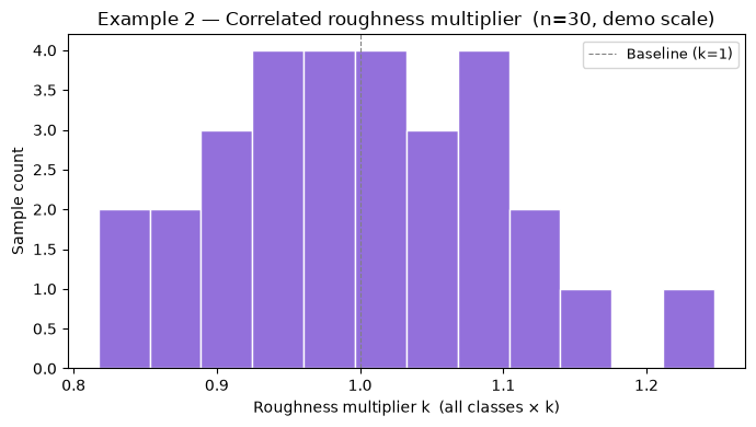
Generated 30 parameter samples; no hydraulic ensemble or driver ranking is established by this cell.

Python

# Build apply_fn: all classes scaled by the shared roughness_multiplier k.
# We use make_mannings_apply_fn with the expanded samples_ex2 (which already
# carries per-class absolute n values = base_n × k for each class).
apply_fn_ex2 = RasMonteCarlo.make_mannings_apply_fn(
    zone_column_map = {name: name for name in lc_names_all},
    path            = "plaintext",
)

# Smart reuse (C-1/C-2/C-3 hardened)
_ex2_batches, _ex2_done_hdfs, _ex2_perm_log = discover_completed_hdfs(project_path, suffix="mc_rough")

_MIN_USABLE_EX2 = (95 * N_SAMPLES_EX2 + 99) // 100  # reuse at >=95% usable (see Ex1)
if len(_ex2_done_hdfs) >= _MIN_USABLE_EX2:
    print(f"Found {len(_ex2_done_hdfs)} completed result HDFs — reusing.")
    ensemble_ex2 = build_reuse_ensemble(_ex2_done_hdfs, N_SAMPLES_EX2, perm_log=_ex2_perm_log)
else:
    if _ex2_batches:
        print(f"Removing {len(_ex2_batches)} incomplete batch folder(s)...")
        for folder in _ex2_batches:
            shutil.rmtree(folder, ignore_errors=True)

    ensemble_ex2 = RasMonteCarlo.run_ensemble(
        template_plan = TEMPLATE_PLAN,
        samples_df    = samples_ex2,     # expanded: per-class columns carry base_n * k
        apply_fn      = apply_fn_ex2,
        suffix        = "mc_rough",
        max_workers   = MAX_WORKERS,
        num_cores     = NUM_CORES,
        timeout_sec   = TIMEOUT_SEC,
        clone_geom    = True,
        clear_geompre = True,
        workers       = remote_workers if USE_REMOTE_WORKERS else None,
    )

report_ensemble_health(ensemble_ex2, "Example 2 (Roughness — secondary driver)")

Python

# Derive representative mesh-cell coordinates for point-level risk analysis.
cells_gdf = HdfMesh.get_mesh_cell_points(TEMPLATE_PLAN, ras_object=ras)

# Sample 4 cells evenly spaced by index to span the domain
n_cells = len(cells_gdf)
step    = max(1, n_cells // 4)
poi_idx = list(range(0, n_cells, step))[:4]
poi_pts = [
    (cells_gdf.geometry.iloc[i].x, cells_gdf.geometry.iloc[i].y)
    for i in poi_idx
]

print(f"Mesh cells available: {n_cells:,}")
print("Points of interest (x, y):")
for j, (x, y) in enumerate(poi_pts):
    print(f"  POI-{j}: ({x:.2f}, {y:.2f})")

# Point-level WSE statistics across completed ensemble members.
# Default min_valid_fraction=0.95 guard applies; status accounting is attached via df.attrs.
risk_df = RasMonteCarlo.risk_at_points(
    ensemble_result = ensemble_ex2,
    points          = poi_pts,
    variable        = "wse",
)

print(f"\nn_samples_used (attrs)  : {risk_df.attrs.get('n_samples_used')}")
print(f"status_accounting (attrs): {risk_df.attrs.get('status_accounting')}")
print("\nPoint-level risk summary:")
display(
    risk_df[["point_index", "x", "y", "n_samples",
             "mean", "std", "p10", "p50", "p90"]].round(3)
)

# Plot WSE percentile curves at each point
fig, ax = plt.subplots(figsize=(9, 5))
pct_cols = ["p01", "p10", "p50", "p90", "p99"]
pct_vals = [1, 10, 50, 90, 99]
colors   = plt.cm.viridis(np.linspace(0.15, 0.85, len(risk_df)))

for (_, row), c in zip(risk_df.iterrows(), colors):
    wse_pcts = [row[col] for col in pct_cols]
    ax.plot(
        pct_vals, wse_pcts,
        marker="o", markersize=5, linewidth=1.6,
        color=c, label=f"POI-{int(row['point_index'])}",
    )

ax.set_xlabel("Percentile (non-exceedance quantile)")
ax.set_ylabel("Water Surface Elevation (ft)")
ax.set_title("Example 2 — Correlated Roughness LHS  |  WSE Percentile Curves at Selected Points")
ax.legend(title="Point of Interest", fontsize=9)
ax.grid(True, alpha=0.35)
plt.tight_layout()
plt.show()

Workflow summary and remaining execution

	Example 1	Example 2
Sampling method	Latin hypercube	Latin hypercube
Parameters	Breach formation (width, time, slopes) + inflow multiplier	Correlated roughness multiplier (all named classes × k)
Ensemble size	100 configured (N_SAMPLES_EX1)	30 configured (N_SAMPLES_EX2)
apply_fn source	make_breach_apply_fn() + make_flow_multiplier_apply_fn()	make_mannings_apply_fn() (shipped factory)
Execution	Remote worker fleet (USE_REMOTE_WORKERS=True)	Local parallel or remote
Ensemble health	status_histogram() after execution	status_histogram() after execution
Convergence	convergence(p90) recipe; no retained finding	Not computed here
Result analysis	exceedance_probabilities() + prediction_intervals()	risk_at_points()

2D Land-Cover Roughness Propagation (Required Settings)

For a 2D land-cover model the roughness MC perturbs the plain-text .g## LCMann Table base overrides through make_mannings_apply_fn(path="plaintext"). This only reaches the solver when run_ensemble() is called with both:

• clone_geom=True -- per-sample geometry, so each sample edits its own .g## LCMann Table.
• clear_geompre=True -- regenerates the cached per-cell Cells Center Manning's n from the perturbed table. Without it the preprocessed n is stale and the ensemble is inert (zero WSE spread).

force_geompre is unnecessary here because clone_geom=True refreshes each .g## mtime; clear_geompre=True therefore runs and clears cached tables in place. Use force_geompre=True for in-place sidecar edits whose unchanged geometry mtime would otherwise trigger the skip.

Public methods used by the full recipe

1. RasMonteCarlo.generate_samples(...) — bounded LHS using the single-threaded default_rng (H5)
2. RasMonteCarlo.make_breach_apply_fn(...) — breach formation parameter perturbation
3. RasMonteCarlo.make_flow_multiplier_apply_fn(...) — inflow QMult scaling
4. RasMonteCarlo.make_composite_apply_fn(...) — chains breach + inflow apply_fns
5. RasMonteCarlo.make_mannings_apply_fn(...) — shipped factory exercised instead of an inline apply_fn (L1)
6. RasMonteCarlo.run_ensemble(...) — returns completed / completed_with_errors / failed + status_histogram (M1)
7. RasMonteCarlo.status_histogram(...) — surfaces ensemble health before statistics (C2)
8. RasMonteCarlo.convergence(...) — running P90 stabilization check (C3)
9. RasMonteCarlo.exceedance_probabilities(...) — default 0.95 valid-fraction guard, status_accounting reported (C2)
10. RasMonteCarlo.prediction_intervals(...) — labelled interval_type="prediction", n_samples_used reported (M3)
11. RasMonteCarlo.risk_at_points(...) — point statistics with n_samples_used / status_accounting in df.attrs (C2)

Limitations

• Sample count alone does not establish quantile adequacy. No hydraulic ensemble or convergence output is retained in this revision. The 100/30 parameter samples are preparation evidence only; study-specific convergence and failed-run sensitivity remain to be evaluated.
• Perfectly correlated roughness scaling (Example 2). One shared multiplier assumes every named land-cover class is biased by the same factor. This preserves hydraulic coupling but does not represent class-specific uncertainty or partial correlation.
• Percentiles are non-exceedance quantiles (value not exceeded by N% of the sampled outcomes), not annual exceedance probabilities, and mix aleatory + epistemic uncertainty in one ensemble.
• Error runs are excluded by default. Runs with status completed_with_errors are dropped from statistics unless include_error_runs=True; the dropped fraction biases the tail and is reported via the status histogram / status_accounting.
• Flow-multiplier note (H2): make_flow_multiplier_apply_fn writes Flow Hydrograph QMult=, a UNIFORM ordinate multiplier scaling peak AND volume together — it is NOT an AEP / flow-frequency sample.
• Sensitivity analysis (Morris/Sobol) is out of scope in this version of RasMonteCarlo.