AORC Precipitation for HEC-RAS Rain-on-Grid Models
This notebook demonstrates a complete workflow for using NOAA's Analysis of Record for Calibration (AORC) gridded precipitation data with HEC-RAS 2D rain-on-grid models, including data-driven simulation buffer selection based on observed watershed response characteristics.
Example Project: BaldEagleCrkMulti2D
Workflow
- Extract example project and create a labeled working copy
- Get project bounds from geometry HDF (with buffer)
- NEW: USGS gauge discovery and watershed response analysis
- Generate a storm catalog with data-driven simulation buffer
- Download precipitation, export hyetographs, and create HEC-RAS plans
- Execute all plans in parallel (2 cores, 3 workers)
- Extract and compare results
- Generate annual downstream boundary condition hydrograph
Key Feature: Data-Driven Simulation Windows
Instead of using an arbitrary 48-hour buffer, this workflow: - Discovers USGS stream gauges in the project area - Retrieves historical flow data for the analysis year - Analyzes watershed response characteristics (time to peak, recession duration) - Calculates recommended buffer based on 90th percentile response time - Ensures simulations capture complete hydrographs (including recession to baseflow)
Data Export
All precipitation data is exported to the Precipitation/ subfolder:
- storm_catalog.csv - Complete storm catalog with metadata
- storm_YYYYMMDD.nc - NetCDF precipitation files
- hyetographs/ - PNG plots of each storm's precipitation
- storm_catalog_summary.png - Overview plot of all storms
- annual_downstream_bc.png - Annual hydrograph from all storm events
- watershed_response_analysis.png - Watershed response time analysis
AORC Dataset Overview
- Coverage: CONUS (1979-present), Alaska (1981-present)
- Resolution: ~800 meters, hourly timesteps
- Format: Cloud-optimized Zarr on AWS S3
- Access: Anonymous (no authentication required)
LLM Forward Approach for Precipitation Data
This notebook demonstrates LLM Forward principles for external precipitation data integration:
- Data Provenance: All AORC data includes:
- NASA/NOAA source metadata (grid resolution, version)
- Retrieval timestamp and data coverage period
-
Storm identification criteria (inter-event hours, minimum depth)
-
Visual Verification: Every step produces reviewable outputs:
- NetCDF files (inspect in Panoply or ncview)
- Storm hyetographs (plot in Excel/Python)
-
Spatial precipitation grids (visualize distribution)
-
Multiple Review Pathways:
- Engineering review (verify storm depths vs regional IDF curves)
- Visual inspection (plot storm catalog, spatial patterns)
-
Data quality checks (grid coverage, missing values)
-
Self-Documenting: Standard folder structure preserves analysis
Precipitation/storm_catalog.csvlists all identified events- Individual NetCDF files preserve raw AORC data
- Hyetograph CSVs enable HEC-HMS/HEC-RAS integration
NOAA AORC Data Standards
Analysis of Record for Calibration (AORC) (NOAA documentation):
- Spatial Resolution: 4 km grid (CONUS coverage)
- Temporal Resolution: Hourly (1979-present)
- Data Source: Stage IV radar + gauge analysis (multi-sensor product)
- Quality Control: NOAA/NWS operational QC procedures
Data Quality Considerations: - AORC represents best-available gridded precipitation - Grid cell size (4 km) may not capture small-scale convective events - Hourly resolution appropriate for watershed response times >2 hours - Consider comparing to local rain gauges for calibration events
When to Use AORC Precipitation
Model Calibration (historical events): - Identify significant storm events from AORC catalog - Extract spatial/temporal precipitation distribution - Use as model input for calibration runs - Compare simulated vs observed hydrographs (see notebook 914)
Continuous Simulation (long-term hydrology): - Download multi-year AORC data (1979-present) - Generate hyetographs for each storm event - Run HEC-RAS in continuous mode - Analyze flood frequency statistics
Regional IDF Curve Validation: - Compare AORC storm depths to Atlas 14 (NOAA point estimates) - Verify spatial averaging effects (4 km grid vs point) - Document differences in engineering analysis
NOT Recommended For: - Small watersheds <1 sq mi (use point rain gauges) - Sub-hourly rainfall analysis (use 5-min gauges) - Real-time flood forecasting (use radar nowcasts)
# Install dependencies (uncomment if needed)
# !pip install ras-commander[precip]  # Includes xarray, zarr, s3fs, netCDF4, rioxarray
# =============================================================================
# DEVELOPMENT MODE TOGGLE
# =============================================================================
USE_LOCAL_SOURCE = False  # <-- TOGGLE THIS

if USE_LOCAL_SOURCE:
    import sys
    from pathlib import Path
    local_path = str(Path.cwd().parent)
    if local_path not in sys.path:
        sys.path.insert(0, local_path)
    print(f"📁 LOCAL SOURCE MODE: Loading from {local_path}/ras_commander")
else:
    print("📦 PIP PACKAGE MODE: Loading installed ras-commander")

# Import ras-commander
from ras_commander import init_ras_project, RasExamples, RasPlan, RasUnsteady, RasCmdr
from ras_commander.precip import PrecipAorc
from ras_commander.hdf.HdfProject import HdfProject

# Additional imports
import os
import shutil
import glob
import pandas as pd
import numpy as np
import matplotlib.pyplot as plt
import xarray as xr

# Verify which version loaded
import ras_commander
print(f"✓ Loaded: {ras_commander.__file__}")
📦 PIP PACKAGE MODE: Loading installed ras-commander
2026-06-11 20:51:17 - numexpr.utils - INFO - NumExpr defaulting to 8 threads.
✓ Loaded: <LOCAL_PATH>\ras_commander\__init__.py
Parameters
Configure these values to customize the notebook for your project.
# =============================================================================
# PARAMETERS - Edit these to customize the notebook
# =============================================================================
from pathlib import Path

# Project Configuration
PROJECT_NAME = "BaldEagleCrkMulti2D"           # Example project to extract
RAS_VERSION = "7.0"               # HEC-RAS version (6.3, 6.5, 6.6, etc.)
SUFFIX = "900"                    # Notebook identifier for project folder

# AORC Settings
ONLINE = True                     # Enable network requests

print(f"Project: {PROJECT_NAME}, Version: {RAS_VERSION}")
Project: BaldEagleCrkMulti2D, Version: 7.0
Step 1: Extract Example Project and Create Working Copy
We extract the BaldEagleCrkMulti2D example and create a labeled copy for our AORC analysis. Note: Existing AORC folders are deleted to ensure repeatability.
# Configuration
YEAR = 2020  # Year to analyze
TEMPLATE_PLAN = "06"  # Template plan with precipitation enabled (DSS-based, version 6.00)
NUM_CORES = 2  # Cores per HEC-RAS instance
MAX_WORKERS = 3  # Parallel worker processes

# Extract base example project
base_project = RasExamples.extract_project(PROJECT_NAME, suffix=SUFFIX)
print(f"Base project extracted to: {base_project}")

# Clean up any existing AORC folders (for repeatability)
print("\nCleaning up existing AORC folders...")
aorc_pattern = base_project.parent / "BaldEagleCrkMulti2D_AORC_*"
existing_folders = list(base_project.parent.glob("BaldEagleCrkMulti2D_AORC_*"))
for folder in existing_folders:
    if folder.is_dir():
        print(f"  Removing: {folder.name}")
        shutil.rmtree(folder)
print(f"  Removed {len(existing_folders)} existing folders")

# Create labeled working copy (include SUFFIX for concurrent testing)
working_folder = base_project.parent / f"BaldEagleCrkMulti2D_AORC_{YEAR}_{SUFFIX}"
print(f"\nCreating working copy: {working_folder}")
shutil.copytree(base_project, working_folder)

# Initialize project
ras = init_ras_project(working_folder, RAS_VERSION)
print(f"\nProject: {ras.project_name}")
print(f"Location: {ras.project_folder}")
print(f"Plans: {len(ras.plan_df)}")
Execution log compacted for commit (31 stream entries, 7132 characters).
Raw executed output is retained in the CLB-894 artifact notebook.
First lines:
  2026-06-11 20:51:23 - ras_commander.RasExamples - INFO - Successfully extracted project 'BaldEagleCrkMulti2D' to <LOCAL_PATH>\examples\example_projects\BaldEagleCrkMulti2D_900
  Base project extracted to: <LOCAL_PATH>\examples\example_projects\BaldEagleCrkMulti2D_900
  Cleaning up existing AORC folders...
    Removing: BaldEagleCrkMulti2D_AORC_2020_900
    Removing: BaldEagleCrkMulti2D_AORC_2020_900 [Worker 1]
    Removing: BaldEagleCrkMulti2D_AORC_2020_900 [Worker 2]
Last lines:
    is available via RasProcess (HEC-RAS 6.6+). See ras_commander/RasProcess.py.
    Remote distributed execution: ras_commander/remote/ (PsExec, Docker, SSH, cloud).
  ═══════════════════════════════════════════════════════════════════════
  Project: BaldEagleDamBrk
  Location: <LOCAL_PATH>\examples\example_projects\BaldEagleCrkMulti2D_AORC_2020_900
  Plans: 11
Step 2: Get Project Bounds from Geometry HDF
Use HdfProject.get_project_bounds_latlon() to extract proper bounds with buffering.
This handles CRS transformation and ensures precipitation coverage.
# Get geometry HDF path from template plan
# The 'Geom File' column contains just the number (e.g., "09"),
# so we need to add the "g" prefix for the geometry file extension
template_row = ras.plan_df[ras.plan_df['plan_number'] == TEMPLATE_PLAN].iloc[0]
geom_number = template_row['Geom File']
geom_hdf = ras.project_folder / f"{ras.project_name}.g{geom_number}.hdf"

print(f"Template plan {TEMPLATE_PLAN} uses geometry: g{geom_number}")
print(f"Geometry HDF: {geom_hdf}")
print(f"Exists: {geom_hdf.exists()}")

# Get bounds with 50% buffer (default)
# This properly handles CRS transformation and includes 2D mesh, 1D elements, and storage areas
bounds = HdfProject.get_project_bounds_latlon(
    geom_hdf,
    buffer_percent=50.0,  # 50% buffer ensures full coverage after reprojection
    include_1d=True,
    include_2d=True,
    include_storage=True
)

west, south, east, north = bounds
print(f"\nProject Bounds (WGS84 with 50% buffer):")
print(f"  West:  {west:.4f}")
print(f"  South: {south:.4f}")
print(f"  East:  {east:.4f}")
print(f"  North: {north:.4f}")
print(f"  Size:  {east-west:.4f} x {north-south:.4f} degrees")
2026-06-11 20:51:24 - ras_commander.hdf.HdfXsec - ERROR - Error processing cross-section data: "Unable to synchronously open object (object 'Polyline Info' doesn't exist)"
2026-06-11 20:51:24 - ras_commander.hdf.HdfXsec - WARNING - No river centerlines found in geometry file
Template plan 06 uses geometry: g09
Geometry HDF: <LOCAL_PATH>\examples\example_projects\BaldEagleCrkMulti2D_AORC_2020_900\BaldEagleDamBrk.g09.hdf
Exists: True

Project Bounds (WGS84 with 50% buffer):
  West:  -77.8672
  South: 40.9044
  East:  -77.2192
  North: 41.2408
  Size:  0.6480 x 0.3364 degrees
Step 2.5: USGS Gauge Discovery and Watershed Response Analysis
Before generating the storm catalog, we analyze actual USGS gauge data to determine how long the watershed takes to respond to precipitation events. This data-driven approach replaces the arbitrary 48-hour buffer with a value based on observed hydrograph characteristics.
Watershed Response Metrics: - Time to Peak: Hours from storm onset to peak flow - Recession Time: Hours from peak flow to return to baseflow - Total Response Time: Time to peak + recession time
Buffer Selection: We use the 90th percentile total response time (rounded up to nearest 12 hours) to ensure simulations capture the complete hydrograph, including the recession limb back to baseflow conditions.
# Find USGS stream gauges within project area
from ras_commander.usgs import UsgsGaugeSpatial, RasUsgsCore

print("Discovering USGS stream gauges in project area...")
print("="*80)

try:
    gauges = UsgsGaugeSpatial.find_gauges_in_project(
        hdf_path=geom_hdf,
        buffer_percent=100.0,  # Larger buffer to find upstream/downstream gauges
        parameter_codes=['00060'],  # Flow (discharge)
        active_only=True
    )

    if len(gauges) > 0:
        print(f"\nFound {len(gauges)} active USGS stream gauge(s):")
        print(gauges[['site_no', 'station_nm', 'drain_area_va', 'dec_lat_va', 'dec_long_va']].to_string(index=False))
    else:
        print("\nNo USGS gauges found in project area")
        print("Will use default 48-hour buffer for simulations")
        gauges = None
except Exception as e:
    print(f"\nError discovering gauges: {e}")
    print("Will use default 48-hour buffer for simulations")
    gauges = None
2026-06-11 20:51:24 - ras_commander.usgs.spatial - INFO - Retrieving project bounds from: <LOCAL_PATH>\examples\example_projects\BaldEagleCrkMulti2D_AORC_2020_900\BaldEagleDamBrk.g09.hdf
2026-06-11 20:51:24 - ras_commander.hdf.HdfXsec - ERROR - Error processing cross-section data: "Unable to synchronously open object (object 'Polyline Info' doesn't exist)"
2026-06-11 20:51:24 - ras_commander.hdf.HdfXsec - WARNING - No river centerlines found in geometry file
2026-06-11 20:51:25 - ras_commander.usgs.spatial - INFO - Querying USGS gauges in bounds: W=-77.975352, S=40.847932, E=-77.110613, N=41.296469
2026-06-11 20:51:25 - ras_commander.usgs.spatial - ERROR - USGS API query failed: get_monitoring_locations() got an unexpected keyword argument 'parameterCd'
Discovering USGS stream gauges in project area...
================================================================================

No USGS gauges found in project area
Will use default 48-hour buffer for simulations
# Retrieve historical flow data for watershed response analysis
usgs_flow_data = {}

if gauges is not None and len(gauges) > 0:
    print("\nRetrieving historical flow data for analysis year...")
    print("="*80)

    for idx, gauge in gauges.iterrows():
        site_no = gauge['site_no']
        station_name = gauge['station_nm']

        try:
            print(f"\n{site_no} - {station_name}")
            print(f"  Querying USGS NWIS for {YEAR}...")

            flow_df = RasUsgsCore.retrieve_flow_data(
                site_no=site_no,
                start_date=f"{YEAR}-01-01",
                end_date=f"{YEAR}-12-31",
                service='iv'  # Instantaneous values (15-min or hourly)
            )

            if flow_df is not None and len(flow_df) > 0:
                usgs_flow_data[site_no] = {
                    'data': flow_df,
                    'station_name': station_name,
                    'drainage_area': gauge.get('drain_area_va', None)
                }
                print(f"  Retrieved {len(flow_df):,} records")
                print(f"  Period: {flow_df.index[0]} to {flow_df.index[-1]}")
                print(f"  Flow range: {flow_df['flow'].min():.1f} - {flow_df['flow'].max():.1f} cfs")
            else:
                print(f"  No data available for {YEAR}")

        except Exception as e:
            print(f"  Error retrieving data: {e}")

    if len(usgs_flow_data) == 0:
        print("\nNo USGS data retrieved - will use default 48-hour buffer")
else:
    print("\nSkipping USGS data retrieval - no gauges found")
Skipping USGS data retrieval - no gauges found
# Analyze watershed response characteristics from USGS flow data
# We detect flow peaks directly to analyze response time BEFORE generating storm catalog

def find_flow_peaks(flow_df, min_peak_flow_quantile=0.75, min_separation_hours=24):
    """
    Identify significant flow peaks in the record for response analysis.

    Parameters
    ----------
    flow_df : pd.DataFrame
        Flow data with DatetimeIndex and 'flow' column
    min_peak_flow_quantile : float
        Minimum flow quantile to consider (0.75 = top 25% of flows)
    min_separation_hours : float
        Minimum hours between peaks

    Returns
    -------
    list : Peak timestamps
    """
    from scipy.signal import find_peaks

    # Find peaks that are significant
    threshold = flow_df['flow'].quantile(min_peak_flow_quantile)
    peaks, properties = find_peaks(
        flow_df['flow'].values,
        height=threshold,
        distance=int(min_separation_hours * 4)  # Assuming 15-min data
    )

    return flow_df.index[peaks].tolist()

def analyze_peak_response(flow_df, peak_time):
    """Analyze response characteristics around a single peak."""

    # Calculate baseflow (pre-peak period)
    pre_peak = flow_df[flow_df.index < peak_time]
    if len(pre_peak) > 100:
        baseflow = pre_peak.tail(1000)['flow'].quantile(0.10)
    else:
        baseflow = flow_df['flow'].quantile(0.10)

    # Find recession (return to 1.2x baseflow)
    recession_threshold = baseflow * 1.2
    post_peak = flow_df[flow_df.index > peak_time]
    below_threshold = post_peak[post_peak['flow'] <= recession_threshold]

    if len(below_threshold) > 0:
        recession_end_time = below_threshold.index[0]
        recession_hours = (recession_end_time - peak_time).total_seconds() / 3600
        returned_to_baseflow = True
    else:
        recession_end_time = flow_df.index[-1]
        recession_hours = (recession_end_time - peak_time).total_seconds() / 3600
        returned_to_baseflow = False

    peak_flow = flow_df.loc[peak_time, 'flow']

    return {
        'peak_time': peak_time,
        'peak_flow': peak_flow,
        'baseflow': baseflow,
        'recession_hours': recession_hours,
        'returned_to_baseflow': returned_to_baseflow
    }

# Analyze all gauges
print("\nAnalyzing watershed response characteristics...")
print("="*80)

all_response_data = []

if len(usgs_flow_data) > 0:
    for site_no, gauge_info in usgs_flow_data.items():
        flow_df = gauge_info['data']
        station_name = gauge_info['station_name']

        print(f"\n{site_no} - {station_name}")

        # Find significant peaks
        peaks = find_flow_peaks(flow_df, min_peak_flow_quantile=0.75, min_separation_hours=48)
        print(f"  Found {len(peaks)} significant flow peaks")

        # Analyze each peak
        for peak_time in peaks:
            response = analyze_peak_response(flow_df, peak_time)
            if response:
                response['site_no'] = site_no
                response['station_name'] = station_name
                all_response_data.append(response)

    # Create response DataFrame
    if all_response_data:
        response_df = pd.DataFrame(all_response_data)

        print(f"\n{'='*80}")
        print(f"Watershed Response Summary ({len(response_df)} events analyzed)")
        print(f"{'='*80}")
        print(f"Avg recession time: {response_df['recession_hours'].mean():.1f} hours")
        print(f"90th percentile recession: {response_df['recession_hours'].quantile(0.90):.1f} hours")
        print(f"Max recession time: {response_df['recession_hours'].max():.1f} hours")
        print(f"Events returning to baseflow: {response_df['returned_to_baseflow'].sum()}/{len(response_df)}")
    else:
        response_df = None
        print("\nNo response data collected")
else:
    response_df = None
    print("\nNo USGS data available for response analysis")
Analyzing watershed response characteristics...
================================================================================

No USGS data available for response analysis
# Calculate recommended simulation buffer from watershed response analysis
print("\nCalculating recommended simulation buffer...")
print("="*80)

if response_df is not None and len(response_df) > 0:
    # Use 90th percentile recession time for safety margin
    # Add typical time-to-peak (assume 12-24 hours for this watershed size)
    p90_recession = response_df['recession_hours'].quantile(0.90)
    typical_time_to_peak = 24  # Conservative estimate for time to peak

    # Total recommended buffer
    recommended_total = p90_recession + typical_time_to_peak

    # Round up to nearest 12 hours for clean simulation intervals
    RESPONSE_BUFFER_HOURS = int(np.ceil(recommended_total / 12) * 12)

    print(f"\nWatershed Response Analysis Results:")
    print(f"  90th percentile recession time: {p90_recession:.1f} hours")
    print(f"  Estimated time to peak: {typical_time_to_peak} hours")
    print(f"  Total response time (90th %-ile): {recommended_total:.1f} hours")
    print(f"\nRecommended Simulation Buffer: {RESPONSE_BUFFER_HOURS} hours")
    print(f"  (Rounded up to nearest 12 hours)")

    if RESPONSE_BUFFER_HOURS > 48:
        print(f"\n  ⚠️  DATA-DRIVEN BUFFER ({RESPONSE_BUFFER_HOURS}h) > DEFAULT BUFFER (48h)")
        print(f"  Simulations will be extended to capture full recession")
        print(f"  Expected runtime increase: ~{RESPONSE_BUFFER_HOURS/48:.1f}x")
    else:
        print(f"\n  ✓ Default 48-hour buffer is sufficient for this watershed")
else:
    # No USGS data - use default
    RESPONSE_BUFFER_HOURS = 48
    print("No USGS response data available")
    print(f"Using default buffer: {RESPONSE_BUFFER_HOURS} hours")

print(f"\n{'='*80}")
print(f"BUFFER CONFIGURATION: {RESPONSE_BUFFER_HOURS} hours before/after storm")
print(f"{'='*80}")
Calculating recommended simulation buffer...
================================================================================
No USGS response data available
Using default buffer: 48 hours

================================================================================
BUFFER CONFIGURATION: 48 hours before/after storm
================================================================================
# Visualize watershed response analysis
if response_df is not None and len(response_df) > 0:
    fig, axes = plt.subplots(2, 2, figsize=(15, 10))

    # Plot 1: Example hydrograph with annotated response
    ax1 = axes[0, 0]
    if len(usgs_flow_data) > 0:
        # Use first gauge for example
        site_no = list(usgs_flow_data.keys())[0]
        flow_df = usgs_flow_data[site_no]['data']
        station_name = usgs_flow_data[site_no]['station_name']

        # Get first analyzed peak for example
        example = response_df.iloc[0]
        peak_time = example['peak_time']

        # Plot 10 days around peak
        plot_start = peak_time - pd.Timedelta(days=3)
        plot_end = peak_time + pd.Timedelta(days=7)
        plot_data = flow_df[(flow_df.index >= plot_start) & (flow_df.index <= plot_end)]

        ax1.plot(plot_data.index, plot_data['flow'], 'b-', linewidth=1.5, label='Observed Flow')
        ax1.axvline(peak_time, color='red', linestyle='--', linewidth=2, label='Peak')
        ax1.axhline(example['baseflow'], color='gray', linestyle=':', linewidth=2, label='Baseflow')
        ax1.axhline(example['baseflow'] * 1.2, color='orange', linestyle=':', linewidth=1.5, label='Recession Threshold (1.2x baseflow)')

        # Add annotation for recession time
        recession_end = peak_time + pd.Timedelta(hours=example['recession_hours'])
        ax1.annotate('', xy=(recession_end, example['peak_flow']*0.5),
                     xytext=(peak_time, example['peak_flow']*0.5),
                     arrowprops=dict(arrowstyle='<->', color='red', lw=2))
        ax1.text((peak_time + (recession_end - peak_time)/2), example['peak_flow']*0.55,
                f"{example['recession_hours']:.0f}h recession",
                ha='center', fontsize=10, fontweight='bold', color='red')

        ax1.set_xlabel('Date/Time', fontsize=11)
        ax1.set_ylabel('Flow (cfs)', fontsize=11)
        ax1.set_title(f'Example Watershed Response\n{station_name}', fontsize=12, fontweight='bold')
        ax1.legend(loc='upper right', fontsize=9)
        ax1.grid(True, alpha=0.3)
        ax1.tick_params(axis='x', rotation=45)

    # Plot 2: Recession time distribution
    ax2 = axes[0, 1]
    ax2.hist(response_df['recession_hours'], bins=20, color='steelblue', alpha=0.8, edgecolor='darkblue')
    ax2.axvline(response_df['recession_hours'].quantile(0.90),
                color='red', linestyle='--', linewidth=2,
                label=f"90th %-ile: {response_df['recession_hours'].quantile(0.90):.0f}h")
    ax2.axvline(RESPONSE_BUFFER_HOURS - typical_time_to_peak,
                color='green', linestyle='--', linewidth=2,
                label=f'Buffer component: {RESPONSE_BUFFER_HOURS - typical_time_to_peak}h')
    ax2.set_xlabel('Recession Time (hours)', fontsize=11)
    ax2.set_ylabel('Count', fontsize=11)
    ax2.set_title('Recession Time Distribution', fontsize=12, fontweight='bold')
    ax2.legend(fontsize=9)
    ax2.grid(True, alpha=0.3, axis='y')

    # Plot 3: Peak flow vs recession time
    ax3 = axes[1, 0]
    for site_no in response_df['site_no'].unique():
        site_data = response_df[response_df['site_no'] == site_no]
        ax3.scatter(site_data['peak_flow'], site_data['recession_hours'],
                   alpha=0.6, s=60, label=site_no)
    ax3.set_xlabel('Peak Flow (cfs)', fontsize=11)
    ax3.set_ylabel('Recession Time (hours)', fontsize=11)
    ax3.set_title('Peak Flow vs Recession Time', fontsize=12, fontweight='bold')
    ax3.legend(fontsize=9)
    ax3.grid(True, alpha=0.3)

    # Plot 4: Response summary by gauge
    ax4 = axes[1, 1]
    gauge_summary = response_df.groupby('site_no').agg({
        'recession_hours': ['mean', 'max'],
        'peak_flow': 'max'
    }).reset_index()
    gauge_summary.columns = ['site_no', 'avg_recession', 'max_recession', 'max_flow']

    x = range(len(gauge_summary))
    ax4.bar(x, gauge_summary['avg_recession'], alpha=0.7, label='Avg Recession', color='steelblue')
    ax4.bar(x, gauge_summary['max_recession'], alpha=0.5, label='Max Recession', color='darkblue')
    ax4.axhline(RESPONSE_BUFFER_HOURS - typical_time_to_peak,
                color='red', linestyle='--', linewidth=2, label=f'Buffer: {RESPONSE_BUFFER_HOURS - typical_time_to_peak}h')
    ax4.set_xlabel('Gauge', fontsize=11)
    ax4.set_ylabel('Recession Time (hours)', fontsize=11)
    ax4.set_title('Response Summary by Gauge', fontsize=12, fontweight='bold')
    ax4.set_xticks(x)
    ax4.set_xticklabels(gauge_summary['site_no'], rotation=45)
    ax4.legend(fontsize=9)
    ax4.grid(True, alpha=0.3, axis='y')

    plt.suptitle(f'Watershed Response Analysis - {YEAR}\n'
                 f'Buffer Selection: {RESPONSE_BUFFER_HOURS} hours '
                 f'(90th %-ile recession + {typical_time_to_peak}h time-to-peak)',
                 fontsize=14, fontweight='bold')
    plt.tight_layout()

    # Save plot
    response_plot_path = precip_folder / "watershed_response_analysis.png"
    plt.savefig(response_plot_path, dpi=150, bbox_inches='tight')
    print(f"\nResponse analysis plot saved to: {response_plot_path}")
    plt.show()
else:
    print("\nNo response analysis to visualize - using default buffer")
No response analysis to visualize - using default buffer
Step 3: Generate Storm Catalog
Analyze AORC data to identify all significant precipitation events for the year.
# Generate storm catalog with data-driven simulation buffer
storm_catalog = PrecipAorc.get_storm_catalog(
    bounds=bounds,
    year=YEAR,
    inter_event_hours=8.0,      # USGS standard for storm separation
    min_depth_inches=0.75,      # Minimum significant precipitation
    buffer_hours=RESPONSE_BUFFER_HOURS  # Data-driven buffer from watershed response analysis
)

print(f"\nStorm Catalog: {len(storm_catalog)} events for {YEAR}")
print(f"Simulation buffer: {RESPONSE_BUFFER_HOURS} hours before/after each storm")
print("="*90)
print(storm_catalog[['storm_id', 'start_time', 'end_time', 'total_depth_in',
                     'peak_intensity_in_hr', 'duration_hours', 'rank']].to_string(index=False))

# Show simulation window duration for context
if len(storm_catalog) > 0:
    avg_sim_duration = (storm_catalog['sim_end'] - storm_catalog['sim_start']).mean()
    avg_sim_hours = avg_sim_duration.total_seconds() / 3600
    print(f"\nAverage simulation duration: {avg_sim_hours:.0f} hours")
    print(f"  (Storm duration + 2 × {RESPONSE_BUFFER_HOURS}h buffer)")
Execution log compacted for commit (12 stream entries, 2802 characters).
Raw executed output is retained in the CLB-894 artifact notebook.
First lines:
  2026-06-11 20:51:25 - ras_commander.precip.PrecipAorc - INFO - Generating storm catalog for 2020
  2026-06-11 20:51:25 - ras_commander.precip.PrecipAorc - INFO -   Bounds: W=-77.8672, S=40.9044, E=-77.2192, N=41.2408
  2026-06-11 20:51:25 - ras_commander.precip.PrecipAorc - INFO -   Parameters: inter_event=8.0h, min_depth=0.75in, buffer=48h
  2026-06-11 20:51:25 - ras_commander.precip.PrecipAorc - INFO - Connecting to AWS S3...
  2026-06-11 20:51:25 - ras_commander.precip.PrecipAorc - INFO - Loading s3://noaa-nws-aorc-v1-1-1km/2020.zarr...
  2026-06-11 20:51:27 - ras_commander.precip.PrecipAorc - INFO - Loading spatial subset...
Last lines:
          9 2020-10-29 07:00:00 2020-10-30 18:00:00           1.735                 0.127              36     5
         10 2020-11-11 12:00:00 2020-11-11 22:00:00           1.989                 0.448              11     3
         11 2020-12-16 17:00:00 2020-12-17 09:00:00           1.834                 0.174              17     4
         12 2020-12-24 12:00:00 2020-12-25 12:00:00           2.720                 0.202              25     1
  Average simulation duration: 116 hours
    (Storm duration + 2 × 48h buffer)
Step 4: Download AORC Data and Export Precipitation Records
Download precipitation data, export storm catalog CSV, and generate hyetograph plots for documentation.
# Create precipitation folder structure
precip_folder = ras.project_folder / "Precipitation"
precip_folder.mkdir(exist_ok=True)
hyetograph_folder = precip_folder / "hyetographs"
hyetograph_folder.mkdir(exist_ok=True)

# Export storm catalog to CSV
catalog_csv = precip_folder / "storm_catalog.csv"
storm_catalog.to_csv(catalog_csv, index=False)
print(f"Storm catalog exported to: {catalog_csv}")

# Download AORC data for all storms
print(f"\nDownloading AORC precipitation data for {len(storm_catalog)} storms...")
print("="*70)

precip_files = {}
for idx, storm in storm_catalog.iterrows():
    storm_id = storm['storm_id']
    date_str = storm['start_time'].strftime('%Y%m%d')
    precip_file = precip_folder / f"storm_{date_str}.nc"

    if not precip_file.exists():
        print(f"  Storm {storm_id:2d}: {storm['start_time'].strftime('%b %d')} - Downloading...")
        PrecipAorc.download(
            bounds=bounds,
            start_time=storm['sim_start'],
            end_time=storm['sim_end'],
            output_path=precip_file,
            target_crs="EPSG:5070",
            resolution=2000.0
        )
    else:
        print(f"  Storm {storm_id:2d}: {storm['start_time'].strftime('%b %d')} - Already downloaded")

    precip_files[storm_id] = precip_file

print(f"\nDownloaded {len(precip_files)} precipitation files to {precip_folder}")
Execution log compacted for commit (157 stream entries, 18058 characters).
Raw executed output is retained in the CLB-894 artifact notebook.
First lines:
  2026-06-11 20:51:29 - ras_commander.precip.PrecipAorc - INFO - Downloading AORC data:
  2026-06-11 20:51:29 - ras_commander.precip.PrecipAorc - INFO -   Bounds: W=-77.8672, S=40.9044, E=-77.2192, N=41.2408
  2026-06-11 20:51:29 - ras_commander.precip.PrecipAorc - INFO -   Time range: 2020-02-05 09:00:00 to 2020-02-09 17:00:00
  2026-06-11 20:51:29 - ras_commander.precip.PrecipAorc - INFO -   Variable: APCP_surface
  2026-06-11 20:51:29 - ras_commander.precip.PrecipAorc - INFO - Connecting to AWS S3...
  2026-06-11 20:51:29 - ras_commander.precip.PrecipAorc - INFO -   Loading year 2020 from s3://noaa-nws-aorc-v1-1-1km/2020.zarr
Last lines:
  2026-06-11 20:51:49 - ras_commander.precip.PrecipAorc - INFO - Combining datasets...
  2026-06-11 20:51:49 - ras_commander.precip.PrecipAorc - INFO - Reprojecting to EPSG:5070 at 2000.0m resolution...
  2026-06-11 20:51:49 - ras_commander.precip.PrecipAorc - INFO - Reprojected grid shape: (144, 24, 30)
  2026-06-11 20:51:49 - ras_commander.precip.PrecipAorc - INFO - Writing to NetCDF: <LOCAL_PATH>\examples\example_projects\BaldEagleCrkMulti2D_AORC_2020_900\Precipitation\storm_20201224.nc
  2026-06-11 20:51:49 - ras_commander.precip.PrecipAorc - INFO - Download complete: <LOCAL_PATH>\examples\example_projects\BaldEagleCrkMulti2D_AORC_2020_900\Precipitation\storm_20201224.nc (0.2 MB)
  Downloaded 12 precipitation files to <LOCAL_PATH>\examples\example_projects\BaldEagleCrkMulti2D_AORC_2020_900\Precipitation
# Generate and save individual hyetograph plots for each storm
print(f"Generating hyetograph plots for {len(storm_catalog)} storms...")
print("="*70)

for idx, storm in storm_catalog.iterrows():
    storm_id = storm['storm_id']
    date_str = storm['start_time'].strftime('%Y%m%d')
    precip_file = precip_files[storm_id]

    # Load precipitation data
    ds = xr.open_dataset(precip_file)
    da = ds['APCP_surface']
    hourly_mean = da.mean(dim=['x', 'y']).values
    times = pd.to_datetime(da.time.values)

    # Create figure
    fig, ax = plt.subplots(figsize=(12, 5))
    ax.bar(times, hourly_mean, width=0.03, color='steelblue', alpha=0.8, edgecolor='darkblue', linewidth=0.5)

    # Add storm info
    ax.set_title(f"Storm {storm_id}: {storm['start_time'].strftime('%B %d, %Y')}\n"
                 f"Total: {storm['total_depth_in']:.2f} in | Peak: {storm['peak_intensity_in_hr']:.3f} in/hr | "
                 f"Duration: {storm['duration_hours']:.0f} hours", fontsize=12, fontweight='bold')
    ax.set_xlabel('Date/Time', fontsize=11)
    ax.set_ylabel('Precipitation Rate (mm/hr)', fontsize=11)
    ax.tick_params(axis='x', rotation=45)
    ax.grid(True, alpha=0.3)

    # Add statistics box
    stats_text = (f"Max Rate: {hourly_mean.max():.2f} mm/hr\n"
                  f"Total: {hourly_mean.sum():.1f} mm\n"
                  f"Timesteps: {len(hourly_mean)}")
    ax.text(0.98, 0.95, stats_text, transform=ax.transAxes, fontsize=9,
            verticalalignment='top', horizontalalignment='right',
            bbox=dict(boxstyle='round', facecolor='wheat', alpha=0.8))

    plt.tight_layout()

    # Save plot
    plot_path = hyetograph_folder / f"storm_{date_str}_hyetograph.png"
    plt.savefig(plot_path, dpi=150, bbox_inches='tight')
    plt.close()

    ds.close()
    print(f"  Storm {storm_id:2d}: {storm['start_time'].strftime('%b %d')} - Saved to {plot_path.name}")

print(f"\nHyetographs saved to: {hyetograph_folder}")
Execution log compacted for commit (13 stream entries, 958 characters).
Raw executed output is retained in the CLB-894 artifact notebook.
First lines:
  Generating hyetograph plots for 12 storms...
  ======================================================================
    Storm  1: Feb 07 - Saved to storm_20200207_hyetograph.png
    Storm  2: Mar 19 - Saved to storm_20200319_hyetograph.png
    Storm  3: Mar 28 - Saved to storm_20200328_hyetograph.png
    Storm  4: Apr 17 - Saved to storm_20200417_hyetograph.png
Last lines:
    Storm  8: Sep 29 - Saved to storm_20200929_hyetograph.png
    Storm  9: Oct 29 - Saved to storm_20201029_hyetograph.png
    Storm 10: Nov 11 - Saved to storm_20201111_hyetograph.png
    Storm 11: Dec 16 - Saved to storm_20201216_hyetograph.png
    Storm 12: Dec 24 - Saved to storm_20201224_hyetograph.png
  Hyetographs saved to: <LOCAL_PATH>\examples\example_projects\BaldEagleCrkMulti2D_AORC_2020_900\Precipitation\hyetographs
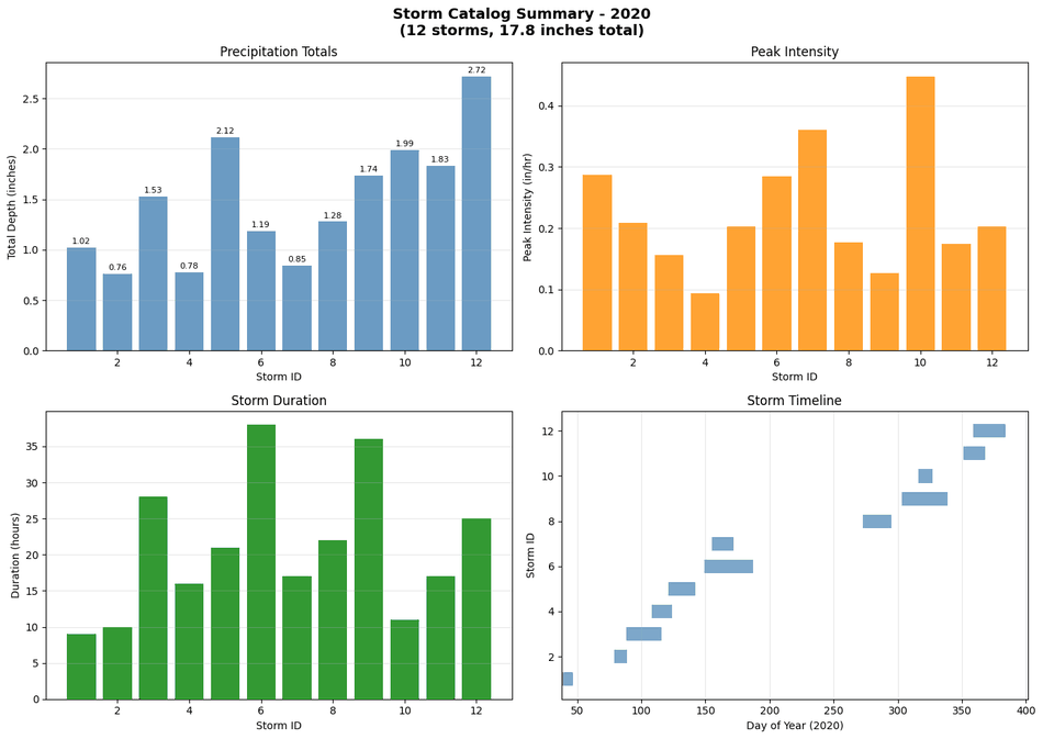
# Create storm catalog summary plot
fig, axes = plt.subplots(2, 2, figsize=(14, 10))

# 1. Total depth by storm
ax1 = axes[0, 0]
bars1 = ax1.bar(storm_catalog['storm_id'], storm_catalog['total_depth_in'], color='steelblue', alpha=0.8)
ax1.set_xlabel('Storm ID')
ax1.set_ylabel('Total Depth (inches)')
ax1.set_title('Precipitation Totals')
ax1.grid(True, alpha=0.3, axis='y')
# Add value labels
for bar, val in zip(bars1, storm_catalog['total_depth_in']):
    ax1.text(bar.get_x() + bar.get_width()/2, bar.get_height() + 0.02, f'{val:.2f}',
             ha='center', va='bottom', fontsize=8)

# 2. Peak intensity
ax2 = axes[0, 1]
bars2 = ax2.bar(storm_catalog['storm_id'], storm_catalog['peak_intensity_in_hr'], color='darkorange', alpha=0.8)
ax2.set_xlabel('Storm ID')
ax2.set_ylabel('Peak Intensity (in/hr)')
ax2.set_title('Peak Intensity')
ax2.grid(True, alpha=0.3, axis='y')

# 3. Duration
ax3 = axes[1, 0]
bars3 = ax3.bar(storm_catalog['storm_id'], storm_catalog['duration_hours'], color='green', alpha=0.8)
ax3.set_xlabel('Storm ID')
ax3.set_ylabel('Duration (hours)')
ax3.set_title('Storm Duration')
ax3.grid(True, alpha=0.3, axis='y')

# 4. Timeline
ax4 = axes[1, 1]
for idx, storm in storm_catalog.iterrows():
    ax4.barh(storm['storm_id'], storm['duration_hours'], left=storm['start_time'].dayofyear,
             color='steelblue', alpha=0.7, height=0.6)
ax4.set_xlabel(f'Day of Year ({YEAR})')
ax4.set_ylabel('Storm ID')
ax4.set_title('Storm Timeline')
ax4.grid(True, alpha=0.3, axis='x')

plt.suptitle(f'Storm Catalog Summary - {YEAR}\n({len(storm_catalog)} storms, '
             f'{storm_catalog["total_depth_in"].sum():.1f} inches total)',
             fontsize=14, fontweight='bold')
plt.tight_layout()

# Save summary plot
summary_path = precip_folder / "storm_catalog_summary.png"
plt.savefig(summary_path, dpi=150, bbox_inches='tight')
print(f"Summary plot saved to: {summary_path}")
plt.show()
Summary plot saved to: <LOCAL_PATH>\examples\example_projects\BaldEagleCrkMulti2D_AORC_2020_900\Precipitation\storm_catalog_summary.png
# Create storm plans with precipitation data written to HDF
print(f"Creating HEC-RAS plans for {len(storm_catalog)} storms...")
print("="*70)

# Use create_storm_plans which calls set_gridded_precipitation
# This writes precipitation data directly to the .u##.hdf file
results = PrecipAorc.create_storm_plans(
    storm_catalog=storm_catalog,
    bounds=bounds,
    template_plan=TEMPLATE_PLAN,
    precip_folder="Precipitation",
    ras_object=ras,
    download_data=False  # Already downloaded above
)

# Show results
print(f"\nPlan Creation Results:")
print(results[['storm_id', 'start_time', 'total_depth_in', 'plan_number', 'status']].to_string(index=False))

# Refresh plan list
ras.plan_df = ras.get_plan_entries()
print(f"\nTotal plans in project: {len(ras.plan_df)}")
Execution log compacted for commit (294 stream entries, 41282 characters).
Raw executed output is retained in the CLB-894 artifact notebook.
First lines:
  2026-06-11 20:51:55 - ras_commander.precip.PrecipAorc - INFO - Creating storm plans from template plan 06 (unsteady 03)
  2026-06-11 20:51:55 - ras_commander.precip.PrecipAorc - INFO -   Precipitation folder: <LOCAL_PATH>\examples\example_projects\BaldEagleCrkMulti2D_AORC_2020_900\Precipitation
  2026-06-11 20:51:55 - ras_commander.precip.PrecipAorc - INFO -   Processing 12 storms
  2026-06-11 20:51:55 - ras_commander.precip.PrecipAorc - INFO - Storm 1: 2020-02-07 (1.02 in)
  2026-06-11 20:51:55 - ras_commander.precip.PrecipAorc - INFO -   Cloning unsteady file...
  2026-06-11 20:51:55 - ras_commander.RasUtils - INFO - File cloned from <LOCAL_PATH>\examples\example_projects\BaldEagleCrkMulti2D_AORC_2020_900\BaldEagleDamBrk.u03 to <LOCAL_PATH>\examples\example_projects\BaldEagleCrkMu
Last lines:
          8 2020-09-29 11:00:00           1.278          16 success
          9 2020-10-29 07:00:00           1.735          20 success
         10 2020-11-11 12:00:00           1.989          21 success
         11 2020-12-16 17:00:00           1.834          22 success
         12 2020-12-24 12:00:00           2.720          23 success
  Total plans in project: 23
Step 5: Execute Storm Plans in Parallel
Run all storm plans using parallel execution with 2 cores per instance and 3 workers.
# Get list of storm plan numbers
storm_plan_numbers = results[results['status'] == 'success']['plan_number'].tolist()
print(f"Plans to execute: {storm_plan_numbers}")
print(f"Execution config: {NUM_CORES} cores x {MAX_WORKERS} workers")
print("="*70)
Plans to execute: ['07', '08', '09', '10', '11', '12', '14', '16', '20', '21', '22', '23']
Execution config: 2 cores x 3 workers
======================================================================
# Execute plans in parallel
import time

print(f"Starting parallel execution of {len(storm_plan_numbers)} plans...")
start_time = time.time()

execution_results = RasCmdr.compute_parallel(
    plan_number=storm_plan_numbers,
    max_workers=MAX_WORKERS,
    num_cores=NUM_CORES,
    ras_object=ras,
    overwrite_dest=True
)

elapsed = time.time() - start_time

# Results summary
success_count = sum(1 for success in execution_results.values() if success)
fail_count = len(execution_results) - success_count

print(f"\nExecution complete in {elapsed/60:.1f} minutes")
print(f"  Successful: {success_count}")
print(f"  Failed: {fail_count}")
print(f"\nResults copied to: {ras.project_folder.parent / (ras.project_folder.name + ' [Computed]')}")
Execution log compacted for commit (157 stream entries, 28309 characters).
Raw executed output is retained in the CLB-894 artifact notebook.
First lines:
  2026-06-11 20:52:19 - ras_commander.RasCmdr - INFO - Filtered plans to execute: ['07', '08', '09', '10', '11', '12', '14', '16', '20', '21', '22', '23']
  2026-06-11 20:52:19 - ras_commander.RasCmdr - INFO - Adjusted max_workers to 3 based on the number of plans to compute: 12
  Starting parallel execution of 12 plans...
  2026-06-11 20:52:19 - ras_commander.RasCmdr - INFO - Created worker folder: <LOCAL_PATH>\examples\example_projects\BaldEagleCrkMulti2D_AORC_2020_900 [Worker 1]
  2026-06-11 20:52:20 - ras_commander.RasMap - INFO - Successfully parsed RASMapper file: <LOCAL_PATH>\examples\example_projects\BaldEagleCrkMulti2D_AORC_2020_900 [Worker 1]\BaldEagleDamBrk.rasmap
  2026-06-11 20:52:20 - ras_commander.RasPrj - INFO - ras-commander v0.98.0 | An open-source project of CLB Engineering Corporation (https://clbengineering.com/) | Docs: https://rascommander.info | GitHub: https://github.c
Last lines:
  2026-06-11 23:55:14 - ras_commander.RasCmdr - INFO - Plan 23: Successful
  2026-06-11 23:55:14 - ras_commander.RasCmdr - INFO - Plan 22: Successful
  Execution complete in 182.9 minutes
    Successful: 12
    Failed: 0
  Results copied to: <LOCAL_PATH>\examples\example_projects\BaldEagleCrkMulti2D_AORC_2020_900 [Computed]
Step 6: Extract and Compare Results
Re-initialize from the computed folder and extract results summary.
# Results are already in original folder (v0.88.1+) - no re-initialization needed

# Extract results summary
import h5py

print("\nStorm Execution Results")
print("="*80)

storm_results = []
for idx, row in results[results['status'] == 'success'].iterrows():
    storm_id = row['storm_id']
    plan_num = row['plan_number']
    exec_success = execution_results.get(plan_num, False)

    plan_row = ras.plan_df[ras.plan_df['plan_number'] == plan_num]
    if len(plan_row) == 0:
        continue

    plan_path = Path(plan_row.iloc[0]['full_path'])
    hdf_path = Path(str(plan_path) + '.hdf')

    result = {
        'storm_id': storm_id,
        'plan_number': plan_num,
        'start_time': row['start_time'],
        'total_depth_in': row['total_depth_in'],
        'exec_success': exec_success,
        'hdf_exists': hdf_path.exists(),
        'hdf_size_mb': hdf_path.stat().st_size / 1e6 if hdf_path.exists() else 0
    }

    # Extract compute time if available
    if hdf_path.exists():
        try:
            with h5py.File(hdf_path, 'r') as f:
                if 'Results/Summary/Compute Processes' in f:
                    cp = f['Results/Summary/Compute Processes'][:]
                    if len(cp) > 0:
                        result['compute_time'] = cp[0]['Compute Time'].decode('utf-8').strip()
        except Exception:
            pass

    storm_results.append(result)
    status = 'OK' if exec_success and result['hdf_exists'] else 'FAILED'
    print(f"Storm {storm_id:2d} ({row['start_time'].strftime('%b %d')}): Plan {plan_num} - {status} - {result['hdf_size_mb']:.1f} MB")

print(f"\nCompleted: {sum(1 for r in storm_results if r['exec_success'])} of {len(storm_results)} storms")
Storm Execution Results
================================================================================
Storm  1 (Feb 07): Plan 07 - OK - 11670.1 MB
Storm  2 (Mar 19): Plan 08 - OK - 11869.9 MB
Storm  3 (Mar 28): Plan 09 - OK - 14850.5 MB
Storm  4 (Apr 17): Plan 10 - OK - 11044.3 MB
Storm  5 (Apr 30): Plan 11 - OK - 12526.2 MB
Storm  6 (May 28): Plan 12 - OK - 13604.4 MB
Storm  7 (Jun 03): Plan 14 - OK - 11301.0 MB
Storm  8 (Sep 29): Plan 16 - OK - 11011.7 MB
Storm  9 (Oct 29): Plan 20 - OK - 14755.5 MB
Storm 10 (Nov 11): Plan 21 - OK - 10602.8 MB
Storm 11 (Dec 16): Plan 22 - OK - 11169.5 MB
Storm 12 (Dec 24): Plan 23 - OK - 14002.0 MB

Completed: 12 of 12 storms
# Display results summary from results_df
# Shows execution status, completion, errors/warnings, and runtime for all plans
desired_cols = ['plan_number', 'plan_title', 'completed', 'has_errors', 'has_warnings', 'runtime_complete_process_hours']
available_cols = [c for c in desired_cols if c in ras.results_df.columns]
ras.results_df[available_cols]
| plan_number | plan_title | completed | has_errors | has_warnings | runtime_complete_process_hours | |
|---|---|---|---|---|---|---|
| 0 | 13 | PMF with Multi 2D Areas | False | False | False | NaN |
| 1 | 15 | 1d-2D Dambreak Refined Grid | False | False | False | NaN |
| 2 | 17 | 2D to 1D No Dam | False | False | False | NaN |
| 3 | 18 | 2D to 2D Run | False | False | False | NaN |
| 4 | 19 | SA to 2D Dam Break Run | False | False | False | NaN |
| 5 | 03 | Single 2D Area - Internal Dam Structure | False | False | False | NaN |
| 6 | 04 | SA to 2D Area Conn - 2D Levee Structure | False | False | False | NaN |
| 7 | 02 | SA to Detailed 2D Breach | False | False | False | NaN |
| 8 | 01 | SA to Detailed 2D Breach FEQ | False | False | False | NaN |
| 9 | 05 | Single 2D area with Bridges FEQ | False | False | False | NaN |
| 10 | 06 | Gridded Precip - Infiltration | False | False | False | NaN |
| 11 | 07 | AORC Storm Feb 07, 2020 | True | False | False | 0.878268 |
| 12 | 08 | AORC Storm Mar 19, 2020 | True | False | False | 0.711272 |
| 13 | 09 | AORC Storm Mar 28, 2020 | True | False | False | 1.048077 |
| 14 | 10 | AORC Storm Apr 17, 2020 | True | False | False | 0.847391 |
| 15 | 11 | AORC Storm Apr 30, 2020 | True | False | False | 0.892678 |
| 16 | 12 | AORC Storm May 28, 2020 | True | False | False | 0.855851 |
| 17 | 14 | AORC Storm Jun 03, 2020 | True | False | False | 0.534657 |
| 18 | 16 | AORC Storm Sep 29, 2020 | True | False | False | 0.567274 |
| 19 | 20 | AORC Storm Oct 29, 2020 | True | False | False | 0.692587 |
| 20 | 21 | AORC Storm Nov 11, 2020 | True | False | False | 0.551719 |
| 21 | 22 | AORC Storm Dec 16, 2020 | True | False | False | 0.656206 |
| 22 | 23 | AORC Storm Dec 24, 2020 | True | False | False | 0.368229 |
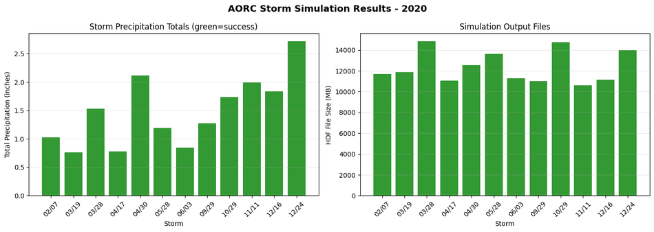
# Summary visualization
if storm_results:
    fig, axes = plt.subplots(1, 2, figsize=(14, 5))

    # Precipitation totals
    ax1 = axes[0]
    storm_dates = [r['start_time'].strftime('%m/%d') for r in storm_results]
    precip_totals = [r['total_depth_in'] for r in storm_results]
    colors = ['green' if r['exec_success'] else 'red' for r in storm_results]

    bars = ax1.bar(range(len(storm_results)), precip_totals, color=colors, alpha=0.8)
    ax1.set_xlabel('Storm')
    ax1.set_ylabel('Total Precipitation (inches)')
    ax1.set_title('Storm Precipitation Totals (green=success)')
    ax1.set_xticks(range(len(storm_results)))
    ax1.set_xticklabels(storm_dates, rotation=45)
    ax1.grid(True, alpha=0.3, axis='y')

    # HDF sizes
    ax2 = axes[1]
    hdf_sizes = [r['hdf_size_mb'] for r in storm_results]
    ax2.bar(range(len(storm_results)), hdf_sizes, color=colors, alpha=0.8)
    ax2.set_xlabel('Storm')
    ax2.set_ylabel('HDF File Size (MB)')
    ax2.set_title('Simulation Output Files')
    ax2.set_xticks(range(len(storm_results)))
    ax2.set_xticklabels(storm_dates, rotation=45)
    ax2.grid(True, alpha=0.3, axis='y')

    plt.suptitle(f'AORC Storm Simulation Results - {YEAR}', fontsize=14, fontweight='bold')
    plt.tight_layout()
    plt.show()
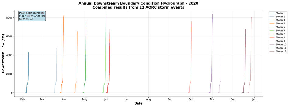
Annual Downstream Boundary Condition Timeline
Extract and combine downstream boundary condition results from all storm simulations to show continuous annual hydrograph.
# Extract downstream boundary condition results from all storm simulations
import h5py
import re

print("Extracting downstream boundary condition results...")
print("="*70)

def parse_hec_time_strings(time_strings):
    """
    Parse HEC-RAS time strings (DDMMMYYYY HH:MM:SS format).

    Args:
        time_strings: Array of byte strings from HDF file

    Returns:
        pd.DatetimeIndex of parsed timestamps
    """
    month_abbr = ['JAN','FEB','MAR','APR','MAY','JUN','JUL','AUG','SEP','OCT','NOV','DEC']
    regex = re.compile(r"(\d{2})([A-Z]{3})(\d{4}) (\d{2}):(\d{2}):(\d{2})")
    parsed_times = []
    for t in time_strings:
        s = t.decode('utf-8')
        m = regex.match(s)
        if m:
            day, mon_ab, year, hour, minute, sec = m.groups()
            mon_num = month_abbr.index(mon_ab.upper()) + 1
            dt = pd.Timestamp(year=int(year), month=mon_num, day=int(day),
                              hour=int(hour), minute=int(minute), second=int(sec))
            parsed_times.append(dt)
        else:
            raise ValueError(f"Could not parse time string: '{s}'")
    return pd.to_datetime(parsed_times)

# Update precip_folder to use computed folder location
precip_folder_computed = ras.project_folder / "Precipitation"
precip_folder_computed.mkdir(exist_ok=True)

# Collect all boundary condition time series
all_bc_data = []

for idx, row in results[results['status'] == 'success'].iterrows():
    storm_id = row['storm_id']
    plan_num = row['plan_number']

    # Skip if execution failed
    if not execution_results.get(plan_num, False):
        continue

    # Get HDF path
    plan_row = ras.plan_df[ras.plan_df['plan_number'] == plan_num]
    if len(plan_row) == 0:
        continue

    plan_path = Path(plan_row.iloc[0]['full_path'])
    hdf_path = Path(str(plan_path) + '.hdf')

    if not hdf_path.exists():
        print(f"  Storm {storm_id:2d}: HDF not found")
        continue

    try:
        with h5py.File(hdf_path, 'r') as f:
            ts_path = 'Results/Unsteady/Output/Output Blocks/Base Output/Unsteady Time Series'

            if ts_path not in f:
                print(f"  Storm {storm_id:2d}: No unsteady time series")
                continue

            # Get timestamps
            times = parse_hec_time_strings(f[f'{ts_path}/Time Date Stamp'][:])

            # Get downstream BC flow from Boundary Conditions
            # DSNormalDepth columns: [Stage, Flow] (from HDF attributes)
            bc_path = f'{ts_path}/Boundary Conditions/DSNormalDepth'
            if bc_path not in f:
                print(f"  Storm {storm_id:2d}: No DSNormalDepth boundary condition")
                continue

            bc_data = f[bc_path][:]
            flow_cfs = bc_data[:, 1]  # Column 1 = Flow (from 'Columns' attribute)

            bc_df = pd.DataFrame({
                'datetime': times,
                'flow_cfs': flow_cfs,
                'storm_id': storm_id
            })
            all_bc_data.append(bc_df)
            print(f"  Storm {storm_id:2d}: {len(times):5d} timesteps, Peak: {flow_cfs.max():8.1f} cfs")

    except Exception as e:
        print(f"  Storm {storm_id:2d}: Error - {e}")

# Combine and plot
if all_bc_data:
    combined_bc = pd.concat(all_bc_data, ignore_index=True)
    combined_bc = combined_bc.sort_values('datetime')

    print(f"\nCombined {len(combined_bc)} timesteps from {len(all_bc_data)} storms")
    print(f"Date range: {combined_bc['datetime'].min()} to {combined_bc['datetime'].max()}")
    print(f"Peak flow: {combined_bc['flow_cfs'].max():.1f} cfs")

    # Create annual plot
    fig, ax = plt.subplots(figsize=(16, 6))

    # Plot each storm with different color
    storm_ids = combined_bc['storm_id'].unique()
    colors = plt.cm.tab20(range(len(storm_ids)))

    for storm_id, color in zip(storm_ids, colors):
        storm_data = combined_bc[combined_bc['storm_id'] == storm_id]
        ax.plot(storm_data['datetime'], storm_data['flow_cfs'],
                color=color, linewidth=1.5, alpha=0.8,
                label=f'Storm {storm_id}')

    # Formatting
    ax.set_xlabel('Date', fontsize=12, fontweight='bold')
    ax.set_ylabel('Downstream Flow (cfs)', fontsize=12, fontweight='bold')
    ax.set_title(f'Annual Downstream Boundary Condition Hydrograph - {YEAR}\n'
                 f'Combined results from {len(storm_ids)} AORC storm events',
                 fontsize=14, fontweight='bold')

    # Format x-axis
    import matplotlib.dates as mdates
    ax.xaxis.set_major_formatter(mdates.DateFormatter('%b'))
    ax.xaxis.set_major_locator(mdates.MonthLocator())

    ax.grid(True, alpha=0.3)
    ax.legend(bbox_to_anchor=(1.02, 1), loc='upper left', fontsize=9)

    # Statistics box
    stats_text = (f"Peak Flow: {combined_bc['flow_cfs'].max():.0f} cfs\n"
                  f"Mean Flow: {combined_bc['flow_cfs'].mean():.0f} cfs\n"
                  f"Events: {len(storm_ids)}")
    ax.text(0.02, 0.98, stats_text, transform=ax.transAxes,
            fontsize=10, verticalalignment='top',
            bbox=dict(boxstyle='round', facecolor='lightblue', alpha=0.8))

    plt.tight_layout()

    # Save figure
    bc_plot_path = precip_folder_computed / "annual_downstream_bc.png"
    plt.savefig(bc_plot_path, dpi=150, bbox_inches='tight')
    print(f"\nAnnual BC plot saved to: {bc_plot_path}")
    plt.show()
else:
    print("\nNo boundary condition data extracted - check HDF file structure")
Extracting downstream boundary condition results...
======================================================================
  Storm  1: 17741 timesteps, Peak:   4298.9 cfs
  Storm  2: 17959 timesteps, Peak:   4722.0 cfs
  Storm  3: 21161 timesteps, Peak:   8204.4 cfs
  Storm  4: 19048 timesteps, Peak:   6534.7 cfs
  Storm  5: 19901 timesteps, Peak:   7535.7 cfs
  Storm  6: 22634 timesteps, Peak:   8370.0 cfs
  Storm  7: 18808 timesteps, Peak:   6724.1 cfs
  Storm  8: 20081 timesteps, Peak:   7611.0 cfs
  Storm  9: 22601 timesteps, Peak:   8366.8 cfs
  Storm 10: 18101 timesteps, Peak:   5117.5 cfs
  Storm 11: 19181 timesteps, Peak:   6743.5 cfs
  Storm 12: 20647 timesteps, Peak:   8022.8 cfs

Combined 237863 timesteps from 12 storms
Date range: 2020-02-05 09:00:00 to 2020-12-27 12:00:00
Peak flow: 8370.0 cfs

Annual BC plot saved to: <LOCAL_PATH>\examples\example_projects\BaldEagleCrkMulti2D_AORC_2020_900\Precipitation\annual_downstream_bc.png
Data Export Summary
All precipitation data has been exported to the project's Precipitation/ folder:
# List all exported files
print(f"Precipitation Data Export Summary")
print(f"Location: {precip_folder}")
print("="*70)

# Count files
nc_files = list(precip_folder.glob("storm_*.nc"))
png_files = list(hyetograph_folder.glob("*.png"))
csv_files = list(precip_folder.glob("*.csv"))
summary_files = list(precip_folder.glob("storm_catalog_summary.png"))
bc_plot_files = list(precip_folder.glob("annual_downstream_bc.png"))

print(f"\nExported Files:")
print(f"  Storm Catalog CSV:    {len(csv_files)} file(s)")
print(f"  NetCDF Precip Files:  {len(nc_files)} file(s)")
print(f"  Hyetograph PNGs:      {len(png_files)} file(s)")
print(f"  Summary Plot:         {len(summary_files)} file(s)")
print(f"  Annual BC Plot:       {len(bc_plot_files)} file(s)")

# Calculate total size
total_size = sum(f.stat().st_size for f in nc_files + png_files + csv_files + summary_files + bc_plot_files)
print(f"\nTotal Size: {total_size / 1e6:.1f} MB")

print(f"\nFolder Structure:")
print(f"  Precipitation/")
print(f"    storm_catalog.csv")
print(f"    storm_catalog_summary.png")
print(f"    annual_downstream_bc.png")
print(f"    storm_YYYYMMDD.nc  (x{len(nc_files)})")
print(f"    hyetographs/")
print(f"      storm_YYYYMMDD_hyetograph.png  (x{len(png_files)})")
Precipitation Data Export Summary
Location: <LOCAL_PATH>\examples\example_projects\BaldEagleCrkMulti2D_AORC_2020_900\Precipitation
======================================================================

Exported Files:
  Storm Catalog CSV:    1 file(s)
  NetCDF Precip Files:  12 file(s)
  Hyetograph PNGs:      12 file(s)
  Summary Plot:         1 file(s)
  Annual BC Plot:       1 file(s)

Total Size: 3.6 MB

Folder Structure:
  Precipitation/
    storm_catalog.csv
    storm_catalog_summary.png
    annual_downstream_bc.png
    storm_YYYYMMDD.nc  (x12)
    hyetographs/
      storm_YYYYMMDD_hyetograph.png  (x12)
Summary
This notebook demonstrated a complete AORC precipitation workflow with data-driven simulation buffer selection:
- Project Setup - Extracted example and created labeled working copy (with cleanup)
- Bounds Calculation - Used
HdfProject.get_project_bounds_latlon()with 50% buffer - Watershed Response Analysis (NEW) - Analyzed USGS gauge data to determine appropriate simulation buffer:
- Discovered USGS stream gauges in project area
- Retrieved historical flow data for analysis year
- Analyzed hydrograph response characteristics (time to peak, recession duration)
- Calculated data-driven buffer based on 90th percentile response time
- Storm Catalog - Generated catalog using USGS standard parameters and data-driven buffer
- Precipitation Export - Downloaded AORC data, exported CSV catalog and hyetograph plots
- Plan Creation - Created HEC-RAS plans with precipitation written to HDF
- Parallel Execution - Ran all plans with 2 cores and 3 workers
- Annual BC Extraction - Combined downstream boundary conditions from all storm events
Key Functions
| Function | Description |
|---|---|
HdfProject.get_project_bounds_latlon() |
Get buffered bounds from geometry HDF |
UsgsGaugeSpatial.find_gauges_in_project() |
Discover USGS gauges in project area |
RasUsgsCore.retrieve_flow_data() |
Retrieve historical flow data for analysis |
PrecipAorc.get_storm_catalog() |
Generate catalog with data-driven buffer |
PrecipAorc.download() |
Download AORC data to NetCDF |
PrecipAorc.create_storm_plans() |
Create plans with precipitation in HDF |
RasCmdr.compute_parallel() |
Execute plans in parallel |
Outputs
The workflow generates comprehensive precipitation and results documentation: - Storm catalog CSV with metadata - Individual storm NetCDF files and hyetographs - Summary plots showing all storms - NEW: Watershed response analysis plot showing data-driven buffer selection rationale - Annual downstream boundary condition hydrograph showing continuous flow response from all AORC events
Data-Driven Buffer Selection
The workflow automatically determines appropriate simulation buffer based on observed watershed response: - Analyzes USGS flow peaks and recession characteristics - Uses 90th percentile recession time + estimated time-to-peak - Falls back to 48-hour default if no USGS data available - Ensures complete hydrograph capture (including recession to baseflow)
Optional: Process All Available AORC Years (1979-2024)
For brevity, the notebook by default only runs years 2020 through 2024
The following cell processes storm catalogs for all available years in the AORC dataset. Each year gets its own project folder with full precipitation data export.
Warning: This can take a very long time and generate many files!
# OPTIONAL: Process all AORC years
# Set PROCESS_ALL_YEARS = True to run

PROCESS_ALL_YEARS = False  # Set to True to process all years

if PROCESS_ALL_YEARS:
    import time

    # AORC is available from 1979-present for CONUS
    ALL_YEARS = list(range(2020, 2024))  # 1979-2024

    print(f"Processing {len(ALL_YEARS)} years of AORC data")
    print(f"Configuration: {NUM_CORES} cores x {MAX_WORKERS} workers per year")
    print(f"Simulation buffer: {RESPONSE_BUFFER_HOURS} hours (data-driven)")
    print("="*80)

    # Clean up ALL existing AORC folders first
    print("\nCleaning up existing AORC folders...")
    existing_folders = list(base_project.parent.glob("BaldEagleCrkMulti2D_AORC_*"))
    for folder in existing_folders:
        if folder.is_dir():
            print(f"  Removing: {folder.name}")
            shutil.rmtree(folder)
    print(f"  Removed {len(existing_folders)} existing folders")

    all_year_results = {}

    for year in ALL_YEARS:
        try:
            print(f"\n{'='*80}")
            print(f"PROCESSING YEAR: {year}")
            print(f"{'='*80}")

            # Create year-specific working folder
            year_folder = base_project.parent / f"BaldEagleCrkMulti2D_AORC_{year}"
            print(f"  Creating: {year_folder.name}")
            shutil.copytree(base_project, year_folder)

            # Initialize
            ras_year = init_ras_project(year_folder, RAS_VERSION)

            # Generate storm catalog with data-driven buffer
            print(f"  Generating storm catalog for {year}...")
            catalog = PrecipAorc.get_storm_catalog(
                bounds=bounds,
                year=year,
                inter_event_hours=8.0,
                min_depth_inches=0.75,
                buffer_hours=RESPONSE_BUFFER_HOURS  # Use data-driven buffer
            )
            print(f"  Found {len(catalog)} storms")

            if len(catalog) == 0:
                print(f"  No storms found for {year}, skipping")
                all_year_results[year] = {'storms': 0, 'plans': 0, 'success': 0, 'elapsed_min': 0}
                continue

            # Create precipitation folder structure
            year_precip_folder = year_folder / "Precipitation"
            year_precip_folder.mkdir(exist_ok=True)
            year_hyetograph_folder = year_precip_folder / "hyetographs"
            year_hyetograph_folder.mkdir(exist_ok=True)

            # Export storm catalog to CSV
            catalog.to_csv(year_precip_folder / "storm_catalog.csv", index=False)
            print(f"  Exported storm catalog CSV")

            # Download precipitation and create plans
            print(f"  Downloading precipitation and creating plans...")
            year_plan_results = PrecipAorc.create_storm_plans(
                storm_catalog=catalog,
                bounds=bounds,
                template_plan=TEMPLATE_PLAN,
                precip_folder="Precipitation",
                ras_object=ras_year,
                download_data=True
            )

            # Generate hyetographs for each storm
            print(f"  Generating hyetograph plots...")
            for idx, storm in catalog.iterrows():
                storm_id = storm['storm_id']
                date_str = storm['start_time'].strftime('%Y%m%d')
                precip_file = year_precip_folder / f"storm_{date_str}.nc"

                if precip_file.exists():
                    ds = xr.open_dataset(precip_file)
                    da = ds['APCP_surface']
                    hourly_mean = da.mean(dim=['x', 'y']).values
                    times = pd.to_datetime(da.time.values)

                    fig, ax = plt.subplots(figsize=(12, 5))
                    ax.bar(times, hourly_mean, width=0.03, color='steelblue', alpha=0.8)
                    ax.set_title(f"Storm {storm_id}: {storm['start_time'].strftime('%B %d, %Y')}\n"
                                 f"Total: {storm['total_depth_in']:.2f} in | Peak: {storm['peak_intensity_in_hr']:.3f} in/hr",
                                 fontsize=12, fontweight='bold')
                    ax.set_xlabel('Date/Time')
                    ax.set_ylabel('Precipitation Rate (mm/hr)')
                    ax.tick_params(axis='x', rotation=45)
                    ax.grid(True, alpha=0.3)
                    plt.tight_layout()
                    plt.savefig(year_hyetograph_folder / f"storm_{date_str}_hyetograph.png", dpi=150, bbox_inches='tight')
                    plt.close()
                    ds.close()

            # Create summary plot
            fig, axes = plt.subplots(1, 3, figsize=(15, 4))
            axes[0].bar(catalog['storm_id'], catalog['total_depth_in'], color='steelblue', alpha=0.8)
            axes[0].set_xlabel('Storm ID')
            axes[0].set_ylabel('Total Depth (in)')
            axes[0].set_title('Precipitation Totals')
            axes[1].bar(catalog['storm_id'], catalog['peak_intensity_in_hr'], color='darkorange', alpha=0.8)
            axes[1].set_xlabel('Storm ID')
            axes[1].set_ylabel('Peak Intensity (in/hr)')
            axes[1].set_title('Peak Intensity')
            axes[2].bar(catalog['storm_id'], catalog['duration_hours'], color='green', alpha=0.8)
            axes[2].set_xlabel('Storm ID')
            axes[2].set_ylabel('Duration (hours)')
            axes[2].set_title('Storm Duration')
            plt.suptitle(f'Storm Catalog Summary - {year}', fontsize=14, fontweight='bold')
            plt.tight_layout()
            plt.savefig(year_precip_folder / "storm_catalog_summary.png", dpi=150, bbox_inches='tight')
            plt.close()

            # Get plan numbers and execute
            plan_numbers = year_plan_results[year_plan_results['status'] == 'success']['plan_number'].tolist()
            print(f"  Created {len(plan_numbers)} plans")

            if len(plan_numbers) == 0:
                print(f"  No successful plans for {year}, skipping execution")
                all_year_results[year] = {'storms': len(catalog), 'plans': 0, 'success': 0, 'elapsed_min': 0}
                continue

            # Execute in parallel
            print(f"  Executing {len(plan_numbers)} plans ({NUM_CORES} cores x {MAX_WORKERS} workers)...")
            start_time = time.time()

            exec_results = RasCmdr.compute_parallel(
                plan_number=plan_numbers,
                max_workers=MAX_WORKERS,
                num_cores=NUM_CORES,
                ras_object=ras_year,
                overwrite_dest=True
            )

            elapsed = time.time() - start_time
            success = sum(1 for v in exec_results.values() if v)

            all_year_results[year] = {
                'storms': len(catalog),
                'plans': len(plan_numbers),
                'success': success,
                'elapsed_min': elapsed / 60
            }

            print(f"  Completed: {success}/{len(plan_numbers)} in {elapsed/60:.1f} minutes")

        except Exception as e:
            print(f"  ERROR processing {year}: {e}")
            all_year_results[year] = {'error': str(e)}

    # Final summary
    print("\n" + "="*80)
    print("ALL YEARS SUMMARY")
    print(f"Buffer used: {RESPONSE_BUFFER_HOURS} hours (data-driven)")
    print("="*80)

    total_storms = 0
    total_success = 0
    for year, res in sorted(all_year_results.items()):
        if 'error' in res:
            print(f"{year}: ERROR - {res['error']}")
        else:
            total_storms += res['storms']
            total_success += res['success']
            print(f"{year}: {res['storms']} storms, {res['success']}/{res['plans']} success, {res['elapsed_min']:.1f} min")

    print(f"\nTOTAL: {total_storms} storms, {total_success} successful simulations")
else:
    print("Set PROCESS_ALL_YEARS = False to process all AORC years (1979-2024)")
    print("Warning: This will take many hours and generate many files!")
    print(f"\nSimulation buffer: {RESPONSE_BUFFER_HOURS} hours (data-driven from watershed response analysis)")
    print("\nEach year will include:")
    print("  - Precipitation/storm_catalog.csv")
    print("  - Precipitation/storm_catalog_summary.png")
    print("  - Precipitation/storm_YYYYMMDD.nc (per storm)")
    print("  - Precipitation/hyetographs/storm_YYYYMMDD_hyetograph.png (per storm)")
Set PROCESS_ALL_YEARS = False to process all AORC years (1979-2024)
Warning: This will take many hours and generate many files!

Simulation buffer: 48 hours (data-driven from watershed response analysis)

Each year will include:
  - Precipitation/storm_catalog.csv
  - Precipitation/storm_catalog_summary.png
  - Precipitation/storm_YYYYMMDD.nc (per storm)
  - Precipitation/hyetographs/storm_YYYYMMDD_hyetograph.png (per storm)