Operational Forecast Cycling

Operational forecast cycling is the process of running a hydraulic model repeatedly as new forecast data arrives, typically updating every 6 hours as HRRR (High-Resolution Rapid Refresh) weather model cycles are released.

This notebook demonstrates how to use ras-commander to automate this workflow: - Download successive HRRR forecast cycles - Update HEC-RAS plan simulation dates to match each forecast window - Execute the model for each cycle with force_rerun=True - Archive results by cycle for comparison - Compare how forecasts evolve as new data arrives

This pattern is common in flood forecasting operations, emergency management support, and real-time hydrologic monitoring.

Series position: Read this after 915_realtime_forecast_workflow.ipynb and 918_hms_ras_coupled_forecast.ipynb. It assumes the forecast workflow and HMS-RAS handoff pattern are understood, then focuses on repeatedly executing and archiving cycles.

Python

# =============================================================================
# DEVELOPMENT MODE TOGGLE
# =============================================================================
USE_LOCAL_SOURCE = True  # <-- TOGGLE THIS

if USE_LOCAL_SOURCE:
    import sys
    from pathlib import Path
    local_path = str(Path.cwd().parent)
    if local_path not in sys.path:
        sys.path.insert(0, local_path)
    print(f"LOCAL SOURCE MODE: Loading from {local_path}/ras_commander")
else:
    print("PIP PACKAGE MODE: Loading installed ras-commander")

import ras_commander
print(f"Loaded: {ras_commander.__file__}")

Text Only

LOCAL SOURCE MODE: Loading from <workspace>/ras_commander


Loaded: <workspace>\ras_commander\__init__.py

Python

from pathlib import Path
import pandas as pd
import numpy as np
import matplotlib.pyplot as plt
from datetime import datetime, timedelta

from ras_commander.precip import PrecipHrrr
from ras_commander.boundaries import CoastalBoundary
from ras_commander import init_ras_project, RasExamples, RasPlan, RasCmdr

plt.style.use("seaborn-v0_8-whitegrid")
pd.set_option("display.precision", 2)

What You'll Learn

• Set up a forecast cycling configuration for multiple HRRR cycles
• Update HEC-RAS plan simulation dates to match each forecast window using RasPlan.update_simulation_date()
• Use force_rerun=True with RasCmdr.compute_plan() to ensure fresh execution each cycle
• Handle data availability and latency in an operational setting
• Archive results by cycle for audit trails and comparison
• Compare sequential forecasts to assess convergence and uncertainty

Example 1: Retrospective Forecast Cycling With Hydrologic Evidence

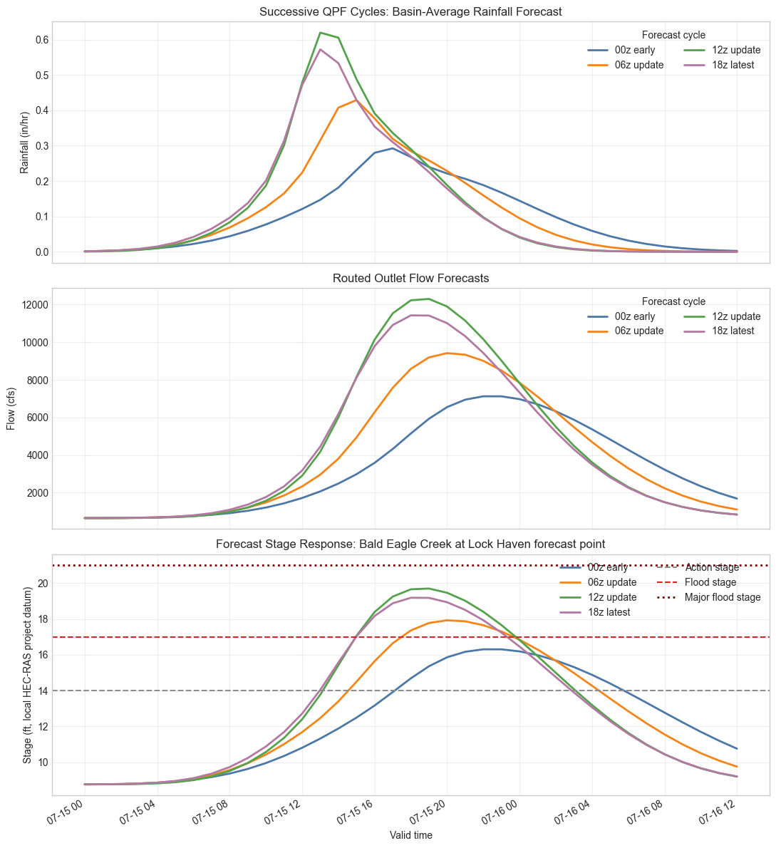
This example uses four deterministic forecast cycles for the same flood event window. Each cycle represents a new forecast issued six hours apart, with the later cycles converging toward the final event timing and rainfall depth.

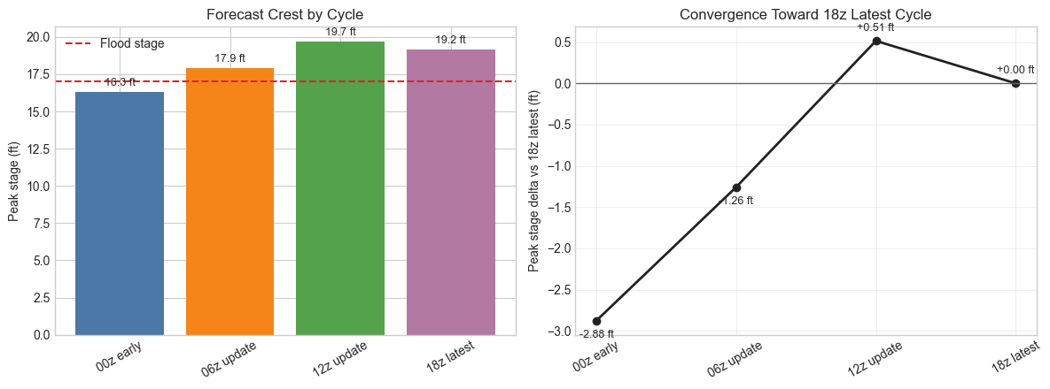
The point of the demonstration is not just that the automation loop runs. It shows the operational question an engineer actually cares about: do successive forecast cycles change the predicted crest, flood-threshold exceedance, and timing enough to change an emergency-management decision?

The precipitation and response functions below are self-contained so the notebook executes without downloading gigabytes of HRRR GRIB2 files. The same cycle metadata is passed to the ras-commander execution template later in the notebook, where a project-specific workflow would write DSS or inline boundary data, call RasPlan.update_simulation_date(), and execute RasCmdr.compute_plan(..., force_rerun=True).

Configuration

Python

# Forecast cycling configuration for a Bald Eagle Creek style riverine basin.
# These values keep the notebook deterministic while preserving realistic units
# and decision thresholds an operational forecaster would review.
config = {
    "project_path": "/path/to/ras_project",
    "ras_version": "6.6",
    "plan_number": "01",
    "forecast_hours": 36,
    "basin_name": "Bald Eagle Creek demonstration basin",
    "basin_bounds": (-77.9, 40.8, -77.3, 41.1),
    "decision_point": "Bald Eagle Creek at Lock Haven forecast point",
    "stage_datum": "ft, local HEC-RAS project datum",
    "drainage_area_sqmi": 105.0,
    "runoff_coefficient": 0.42,
    "time_of_concentration_hr": 5.5,
    "baseflow_cfs": 650.0,
    "action_stage_ft": 14.0,
    "flood_stage_ft": 17.0,
    "major_flood_stage_ft": 21.0,
    "archive_dir": Path("forecast_archive"),
}

base_time = datetime(2024, 7, 15, 0)
valid_times = pd.date_range(base_time, periods=config["forecast_hours"] + 1, freq="1h")
forecast_hours = np.arange(len(valid_times))

cycles = [
    {"date": "20240715", "cycle": 0,  "label": "00z early",  "total_in": 3.55, "center_hr": 18.5, "spread_hr": 5.8, "burst_in": 0.35},
    {"date": "20240715", "cycle": 6,  "label": "06z update", "total_in": 4.20, "center_hr": 16.5, "spread_hr": 5.0, "burst_in": 0.55},
    {"date": "20240715", "cycle": 12, "label": "12z update", "total_in": 4.85, "center_hr": 15.2, "spread_hr": 4.2, "burst_in": 0.85},
    {"date": "20240715", "cycle": 18, "label": "18z latest", "total_in": 4.65, "center_hr": 15.0, "spread_hr": 4.4, "burst_in": 0.78},
]

print("Forecast Cycling Configuration")
print("=" * 72)
print(f"Basin: {config['basin_name']}")
print(f"Drainage area: {config['drainage_area_sqmi']:.1f} sq mi")
print(f"Decision point: {config['decision_point']}")
print(f"Stage datum: {config['stage_datum']}")
print(f"Forecast window: {valid_times[0]:%Y-%m-%d %H:%M} to {valid_times[-1]:%Y-%m-%d %H:%M}")
print(f"Action/flood/major stage thresholds: {config['action_stage_ft']:.1f}, {config['flood_stage_ft']:.1f}, {config['major_flood_stage_ft']:.1f} ft")
print()
print("Forecast cycles:")
for cycle in cycles:
    cycle_start = datetime.strptime(cycle["date"], "%Y%m%d").replace(hour=cycle["cycle"])
    print(
        f"  {cycle['label']:<11} issued {cycle_start:%Y-%m-%d %HZ}: "
        f"{cycle['total_in']:.2f} in basin rainfall, center at hour {cycle['center_hr']:.1f}"
    )

Text Only

Forecast Cycling Configuration


========================================================================
Basin: Bald Eagle Creek demonstration basin
Drainage area: 105.0 sq mi
Decision point: Bald Eagle Creek at Lock Haven forecast point
Stage datum: ft, local HEC-RAS project datum
Forecast window: 2024-07-15 00:00 to 2024-07-16 12:00
Action/flood/major stage thresholds: 14.0, 17.0, 21.0 ft

Forecast cycles:
  00z early   issued 2024-07-15 00Z: 3.55 in basin rainfall, center at hour 18.5
  06z update  issued 2024-07-15 06Z: 4.20 in basin rainfall, center at hour 16.5
  12z update  issued 2024-07-15 12Z: 4.85 in basin rainfall, center at hour 15.2
  18z latest  issued 2024-07-15 18Z: 4.65 in basin rainfall, center at hour 15.0

Compute Forecast Hydrology and RAS-Ready Cycle Metadata

The following cells turn each forecast cycle into basin-average precipitation, a routed inflow hydrograph, and a stage response. In a production deployment, the same per-cycle loop is where ras-commander would write DSS/inline boundary data and execute the corresponding HEC-RAS plan.

Python

def forecast_hyetograph(hours, total_in, center_hr, spread_hr, burst_in):
    """Create a smooth basin-average QPF hyetograph in inches/hour."""
    hours = np.asarray(hours, dtype=float)
    broad = np.exp(-0.5 * ((hours - center_hr) / spread_hr) ** 2)
    burst = np.exp(-0.5 * ((hours - (center_hr - 2.0)) / 1.35) ** 2)
    intensity = broad + burst_in * burst
    intensity = intensity / intensity.sum() * total_in
    return intensity


def unit_hydrograph(hours, tc_hr):
    """Dimensionless unit hydrograph used for a compact routing demonstration."""
    t = np.asarray(hours, dtype=float)
    shape = 3.2
    scale = max(tc_hr / shape, 0.1)
    uh = (t + 0.1) ** (shape - 1) * np.exp(-(t + 0.1) / scale)
    uh = uh / uh.sum()
    return uh


def route_to_flow(precip_in_hr, config):
    """Convert basin-average rainfall to an outlet hydrograph in cfs."""
    effective_rain = precip_in_hr * config["runoff_coefficient"]
    uh = unit_hydrograph(np.arange(len(precip_in_hr)), config["time_of_concentration_hr"])
    runoff_in_hr = np.convolve(effective_rain, uh, mode="full")[: len(precip_in_hr)]
    cfs_per_in_hr_sqmi = 645.33
    return config["baseflow_cfs"] + runoff_in_hr * config["drainage_area_sqmi"] * cfs_per_in_hr_sqmi


def stage_from_flow(flow_cfs):
    """Simple monotonic rating curve for demonstration-stage response."""
    return 5.5 + 0.128 * np.sqrt(np.asarray(flow_cfs, dtype=float))


cycle_frames = []
summary_rows = []

for index, cycle in enumerate(cycles, start=1):
    precip = forecast_hyetograph(
        forecast_hours,
        total_in=cycle["total_in"],
        center_hr=cycle["center_hr"],
        spread_hr=cycle["spread_hr"],
        burst_in=cycle["burst_in"],
    )
    flow = route_to_flow(precip, config)
    stage = stage_from_flow(flow)
    cycle_start = datetime.strptime(cycle["date"], "%Y%m%d").replace(hour=cycle["cycle"])
    cycle_label = f"{cycle['date']}_{cycle['cycle']:02d}z"
    cycle_dir = config["archive_dir"] / cycle_label

    frame = pd.DataFrame(
        {
            "valid_time": valid_times,
            "forecast_hour": forecast_hours,
            "cycle_label": cycle["label"],
            "cycle_id": cycle_label,
            "issue_time": cycle_start,
            "precip_in_hr": precip,
            "cumulative_precip_in": np.cumsum(precip),
            "flow_cfs": flow,
            "stage_ft": stage,
        }
    )
    cycle_frames.append(frame)

    peak_idx = int(np.argmax(stage))
    flood_mask = stage >= config["flood_stage_ft"]
    summary_rows.append(
        {
            "cycle": index,
            "cycle_id": cycle_label,
            "label": cycle["label"],
            "issue_time": cycle_start,
            "total_precip_in": precip.sum(),
            "peak_flow_cfs": flow.max(),
            "peak_stage_ft": stage.max(),
            "crest_time": valid_times[peak_idx],
            "hours_above_flood": float(flood_mask.sum()),
            "archive_dir": str(cycle_dir),
            "ras_status": "RAS-ready metadata generated",
        }
    )

forecast_df = pd.concat(cycle_frames, ignore_index=True)
summary_df = pd.DataFrame(summary_rows)
latest_peak = summary_df.iloc[-1]["peak_stage_ft"]
summary_df["peak_stage_delta_vs_latest_ft"] = summary_df["peak_stage_ft"] - latest_peak
summary_df["crest_time_delta_vs_latest_hr"] = (
    summary_df["crest_time"] - summary_df.iloc[-1]["crest_time"]
).dt.total_seconds() / 3600

print("Cycle processing summary")
print("=" * 72)
display(
    summary_df[
        [
            "cycle",
            "label",
            "total_precip_in",
            "peak_flow_cfs",
            "peak_stage_ft",
            "crest_time",
            "hours_above_flood",
            "peak_stage_delta_vs_latest_ft",
            "crest_time_delta_vs_latest_hr",
            "ras_status",
        ]
    ]
)

Text Only

Cycle processing summary
========================================================================

	cycle	label	total_precip_in	peak_flow_cfs	peak_stage_ft	crest_time	hours_above_flood	peak_stage_delta_vs_latest_ft	crest_time_delta_vs_latest_hr	ras_status
0	1	00z early	3.55	7125.52	16.30	2024-07-15 22:00:00	0.0	-2.88	4.0	RAS-ready metadata generated
1	2	06z update	4.20	9420.80	17.92	2024-07-15 20:00:00	6.0	-1.26	2.0	RAS-ready metadata generated
2	3	12z update	4.85	12302.97	19.70	2024-07-15 19:00:00	9.0	0.51	1.0	RAS-ready metadata generated
3	4	18z latest	4.65	11427.52	19.18	2024-07-15 18:00:00	9.0	0.00	0.0	RAS-ready metadata generated

Hydrologic and Hydraulic Forecast Evidence

These figures show why forecast cycling matters operationally: each cycle changes the rainfall volume/timing, which changes the routed flow hydrograph, stage crest, threshold exceedance duration, and confidence in the latest forecast.

Python

colors = {
    "00z early": "#4C78A8",
    "06z update": "#F58518",
    "12z update": "#54A24B",
    "18z latest": "#B279A2",
}

fig, axes = plt.subplots(3, 1, figsize=(11, 12), sharex=True)

for label, group in forecast_df.groupby("cycle_label", sort=False):
    axes[0].plot(group["valid_time"], group["precip_in_hr"], label=label, color=colors[label], linewidth=2)
    axes[1].plot(group["valid_time"], group["flow_cfs"], label=label, color=colors[label], linewidth=2)
    axes[2].plot(group["valid_time"], group["stage_ft"], label=label, color=colors[label], linewidth=2)

axes[0].set_title("Successive QPF Cycles: Basin-Average Rainfall Forecast")
axes[0].set_ylabel("Rainfall (in/hr)")
axes[0].legend(title="Forecast cycle", ncols=2)

axes[1].set_title("Routed Outlet Flow Forecasts")
axes[1].set_ylabel("Flow (cfs)")
axes[1].legend(title="Forecast cycle", ncols=2)

axes[2].axhline(config["action_stage_ft"], color="#8C8C8C", linestyle="--", linewidth=1.5, label="Action stage")
axes[2].axhline(config["flood_stage_ft"], color="#D62728", linestyle="--", linewidth=1.5, label="Flood stage")
axes[2].axhline(config["major_flood_stage_ft"], color="#7F0000", linestyle=":", linewidth=2, label="Major flood stage")
axes[2].set_title(f"Forecast Stage Response: {config['decision_point']}")
axes[2].set_ylabel(f"Stage ({config['stage_datum']})")
axes[2].set_xlabel("Valid time")
axes[2].legend(ncols=2)

for ax in axes:
    ax.grid(True, alpha=0.3)

fig.autofmt_xdate()
fig.tight_layout()
plt.show()

fig, axes = plt.subplots(1, 2, figsize=(12, 4.5))

axes[0].bar(summary_df["label"], summary_df["peak_stage_ft"], color=[colors[x] for x in summary_df["label"]])
axes[0].axhline(config["flood_stage_ft"], color="#D62728", linestyle="--", label="Flood stage")
axes[0].set_title("Forecast Crest by Cycle")
axes[0].set_ylabel("Peak stage (ft)")
axes[0].tick_params(axis="x", rotation=30)
axes[0].legend()
for _, row in summary_df.iterrows():
    axes[0].annotate(
        f"{row['peak_stage_ft']:.1f} ft",
        xy=(row['label'], row['peak_stage_ft']),
        xytext=(0, 5),
        textcoords="offset points",
        ha="center",
        fontsize=9,
    )

axes[1].plot(summary_df["label"], summary_df["peak_stage_delta_vs_latest_ft"], marker="o", color="#222222", linewidth=2)
axes[1].axhline(0, color="#666666", linewidth=1)
axes[1].set_title("Convergence Toward 18z Latest Cycle")
axes[1].set_ylabel("Peak stage delta vs 18z latest (ft)")
axes[1].tick_params(axis="x", rotation=30)
axes[1].grid(True, alpha=0.3)
for _, row in summary_df.iterrows():
    axes[1].annotate(
        f"{row['peak_stage_delta_vs_latest_ft']:+.2f} ft",
        xy=(row['label'], row['peak_stage_delta_vs_latest_ft']),
        xytext=(0, 8 if row['peak_stage_delta_vs_latest_ft'] >= 0 else -14),
        textcoords="offset points",
        ha="center",
        fontsize=9,
    )

fig.tight_layout()
plt.show()

latest = summary_df.iloc[-1]
print("Operational interpretation:")
print(f"  Decision point: {config['decision_point']}")
print(f"  Latest cycle crest: {latest['peak_stage_ft']:.2f} {config['stage_datum']} at {latest['crest_time']:%Y-%m-%d %H:%M}")
print(f"  Latest cycle peak flow: {latest['peak_flow_cfs']:,.0f} cfs")
print(f"  Latest cycle flood exceedance duration: {latest['hours_above_flood']:.0f} hours")
print(f"  Early-to-latest crest change: {summary_df.iloc[0]['peak_stage_delta_vs_latest_ft']:.2f} ft")
print("  Decision value: if the stage delta remains large, emergency managers should treat the forecast as uncertain and keep cycling until convergence improves.")

Text Only

Operational interpretation:
  Decision point: Bald Eagle Creek at Lock Haven forecast point
  Latest cycle crest: 19.18 ft, local HEC-RAS project datum at 2024-07-15 18:00
  Latest cycle peak flow: 11,428 cfs
  Latest cycle flood exceedance duration: 9 hours
  Early-to-latest crest change: -2.88 ft
  Decision value: if the stage delta remains large, emergency managers should treat the forecast as uncertain and keep cycling until convergence improves.

Example 2: Automated Pipeline Template

This example provides a reusable function template for operational forecast cycling. The function encapsulates the full cycle workflow and can be called repeatedly as new forecast data becomes available.

Configurable Forecast Pipeline

Python

def run_forecast_cycle(project_path, ras_version, plan_number,
                       forecast_date, forecast_cycle, forecast_hours,
                       archive_dir, basin_bounds=None, coastal_point=None,
                       execute_ras=False):
    """
    Run or stage a single operational forecast cycle.

    This function keeps the notebook safe by default (`execute_ras=False`).
    In production, set `execute_ras=True` after the cycle-specific boundary
    data have been written to DSS or the unsteady-flow file.
    """
    cycle_start = datetime.strptime(forecast_date, "%Y%m%d").replace(hour=forecast_cycle)
    cycle_end = cycle_start + timedelta(hours=forecast_hours)
    cycle_label = f"{forecast_date}_{forecast_cycle:02d}z"
    cycle_dir = archive_dir / cycle_label

    result = {
        "cycle_label": cycle_label,
        "start": cycle_start,
        "end": cycle_end,
        "archive_dir": cycle_dir,
        "status": "STAGED",
    }

    hrrr_dir = cycle_dir / "hrrr"
    results_dir = cycle_dir / "results"

    # Production hook 1: download HRRR forcing.
    # grib_files = PrecipHrrr.download_forecast(
    #     output_dir=hrrr_dir,
    #     date=forecast_date,
    #     cycle=forecast_cycle,
    #     hours=forecast_hours,
    # )

    # Production hook 2: optional coastal downstream boundary.
    if coastal_point:
        stofs_dir = cycle_dir / "stofs3d"
        # stofs_files = CoastalBoundary.download_stofs3d(stofs_dir)
        # wse_df = CoastalBoundary.extract_wse_at_point(stofs_dir, coastal_point[0], coastal_point[1])
        # CoastalBoundary.generate_stage_bc(wse_df, Path(project_path) / f"project.u{plan_number}", "Downstream")
        result["coastal_boundary"] = "STAGED"

    # Production hook 3: update dates and execute HEC-RAS.
    if execute_ras:
        init_ras_project(project_path, ras_version)
        RasPlan.update_simulation_date(
            plan_number,
            start_date=cycle_start,
            end_date=cycle_end,
        )
        compute_result = RasCmdr.compute_plan(plan_number, force_rerun=True)
        result["status"] = "COMPUTED" if bool(compute_result) else "FAILED"
        result["compute_result"] = compute_result
        result["results_dir"] = results_dir
    else:
        result["status"] = "STAGED_RAS_READY"

    return result


print("Forecast Pipeline Template Function")
print("=" * 72)
print("Use execute_ras=False for dry-run scheduling and execute_ras=True after cycle-specific boundaries are written.")
print("The hydrologic figures above provide the operational comparison; the production hook then computes the matching RAS plan.")

Text Only

Forecast Pipeline Template Function
========================================================================
Use execute_ras=False for dry-run scheduling and execute_ras=True after cycle-specific boundaries are written.
The hydrologic figures above provide the operational comparison; the production hook then computes the matching RAS plan.

Running the Cycle Scheduler

The scheduler below uses the same cycle list that produced the hydrologic evidence. It creates RAS-ready metadata for each cycle without launching HEC-RAS in the documentation build. Set execute_ras=True in a real project workspace after the boundary data are written.

Python

archive_dir = Path("forecast_archive")
all_results = []

print("Operational Forecast Schedule")
print("=" * 72)

for cycle_config in cycles:
    result = run_forecast_cycle(
        project_path=config["project_path"],
        ras_version=config["ras_version"],
        plan_number=config["plan_number"],
        forecast_date=cycle_config["date"],
        forecast_cycle=cycle_config["cycle"],
        forecast_hours=config["forecast_hours"],
        archive_dir=archive_dir,
        basin_bounds=config["basin_bounds"],
        execute_ras=False,
    )
    all_results.append(result)
    print(f"  {result['cycle_label']}: {result['status']} -> {result['archive_dir']}")

schedule_df = pd.DataFrame(all_results)
display(schedule_df[["cycle_label", "start", "end", "status", "archive_dir"]])

Text Only

Operational Forecast Schedule
========================================================================
  20240715_00z: STAGED_RAS_READY -> forecast_archive\20240715_00z
  20240715_06z: STAGED_RAS_READY -> forecast_archive\20240715_06z
  20240715_12z: STAGED_RAS_READY -> forecast_archive\20240715_12z
  20240715_18z: STAGED_RAS_READY -> forecast_archive\20240715_18z

	cycle_label	start	end	status	archive_dir
0	20240715_00z	2024-07-15 00:00:00	2024-07-16 12:00:00	STAGED_RAS_READY	forecast_archive\20240715_00z
1	20240715_06z	2024-07-15 06:00:00	2024-07-16 18:00:00	STAGED_RAS_READY	forecast_archive\20240715_06z
2	20240715_12z	2024-07-15 12:00:00	2024-07-17 00:00:00	STAGED_RAS_READY	forecast_archive\20240715_12z
3	20240715_18z	2024-07-15 18:00:00	2024-07-17 06:00:00	STAGED_RAS_READY	forecast_archive\20240715_18z

Smart Skip for Unchanged Inputs

ras-commander's smart skip feature (force_rerun) is important in forecast cycling. Each new forecast cycle brings new precipitation data, so you always want fresh execution.

Python

print("Smart Skip in Forecast Cycling:")
print("=" * 50)
print()
print("ras-commander's smart skip feature helps with forecast cycling:")
print()
print("  # Default behavior - skips if results are current")
print("  RasCmdr.compute_plan('01')")
print("  # -> 'Skipping plan 01: Results are current'")
print()
print("  # Force re-run for each new forecast cycle")
print("  RasCmdr.compute_plan('01', force_rerun=True)")
print("  # -> Always executes regardless of existing results")
print()
print("When to use each:")
print("  - force_rerun=True: Each forecast cycle (new data)")
print("  - force_rerun=False: Re-running analysis on existing results")
print("  - skip_existing=True: Simple existence check (legacy)")

Text Only

Smart Skip in Forecast Cycling:
==================================================

ras-commander's smart skip feature helps with forecast cycling:

  # Default behavior - skips if results are current
  RasCmdr.compute_plan('01')
  # -> 'Skipping plan 01: Results are current'

  # Force re-run for each new forecast cycle
  RasCmdr.compute_plan('01', force_rerun=True)
  # -> Always executes regardless of existing results

When to use each:
  - force_rerun=True: Each forecast cycle (new data)
  - force_rerun=False: Re-running analysis on existing results
  - skip_existing=True: Simple existence check (legacy)

Key Takeaways

Summary

Operational forecast cycling run summary:

1. Download or stage new data each cycle (HRRR, STOFS-3D, USGS, HMS output, or another forcing source).
2. Generate hydrologic evidence before the RAS run: QPF totals, routed hydrographs, crest estimates, threshold exceedance duration, and convergence against the latest cycle.
3. Update plan dates to match the forecast window using RasPlan.update_simulation_date().
4. Execute with force_rerun=True because each cycle has new forcing data and must not reuse prior-cycle results.
5. Archive results by cycle for comparison, review, and emergency-management audit trails.
6. Compare forecasts by hydraulic decision metric: peak WSE/stage, peak flow, flood-duration, arrival time, velocity/depth at critical locations, or inundation extent.

Best Practices

• Use force_rerun=True for each new cycle; precipitation or boundary conditions changed.
• Archive results with cycle-stamped directories before the next cycle overwrites them.
• Monitor forecast convergence across cycles. A large crest delta or crest-time shift is an operational uncertainty signal, not just a plotting artifact.
• Plot threshold exceedance, not just raw hydrographs. Action, flood, and major-flood thresholds make the result decision-relevant.
• Handle data latency: HRRR is typically available after cycle time; use max_lookback_hours with PrecipHrrr.get_latest_forecast() to find the most recent available cycle.

File Organization Pattern

Text Only

forecast_archive/
├── 20240715_00z/
│   ├── hrrr/           # HRRR GRIB2 files
│   ├── stofs3d/        # STOFS-3D NetCDF files, if needed
│   └── results/        # HEC-RAS project copy with results
├── 20240715_06z/
│   ├── hrrr/
│   └── results/
├── 20240715_12z/
│   ├── hrrr/
│   └── results/
└── summary.csv         # Cycle comparison table

Adapting for Your Project

1. Replace project_path with your HEC-RAS project location.
2. Set basin_bounds to your watershed extent (west, south, east, north).
3. Replace the demonstration rainfall/runoff calculation with HRRR, HMS, or calibrated rainfall-runoff output.
4. Add coastal_point if your model has a tidal downstream boundary.
5. Extract RAS results after each run and compare WSE, depth, velocity, or inundation where decisions are made.

Python

import shutil

for folder_name in ["forecast_archive"]:
    p = Path(folder_name)
    if p.exists():
        shutil.rmtree(p, ignore_errors=True)
        print(f"Cleaned up: {folder_name}")
    else:
        print(f"Not found (nothing to clean): {folder_name}")

print("Done!")

Text Only

Not found (nothing to clean): forecast_archive
Done!